PCB Coaxial-Fed Horn Antenna (3-7 GHz)

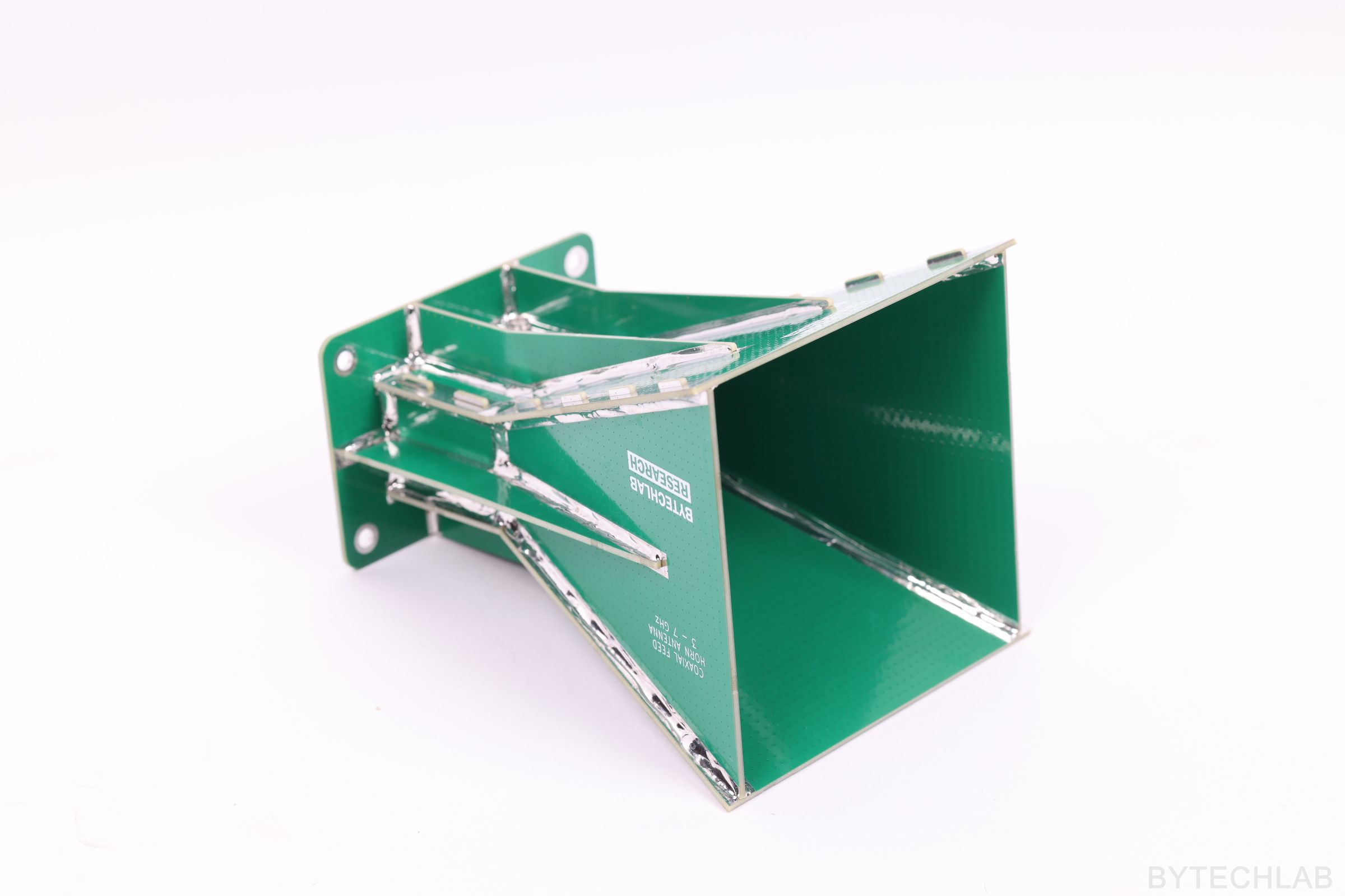
I have designed this antenna mainly because I need a lot of good antennas for my radar projects / experiments – I have quickly realized that my 3D Printed Double Ridged Horn Antenna that I have designed and built previously is not quick / easy / cheap to make. I started to look for good alternatives for 5.8 GHz ISM band, after comparing lots of different designs I have finally decided to move forward with this PCB Coaxial-Fed Horn Antenna.

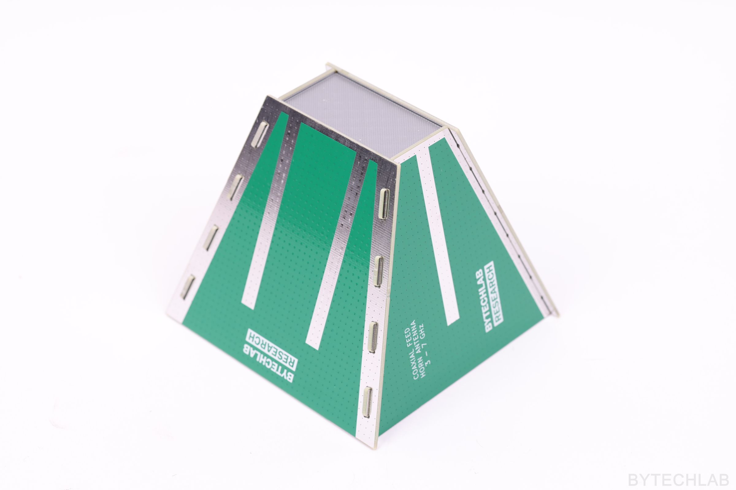
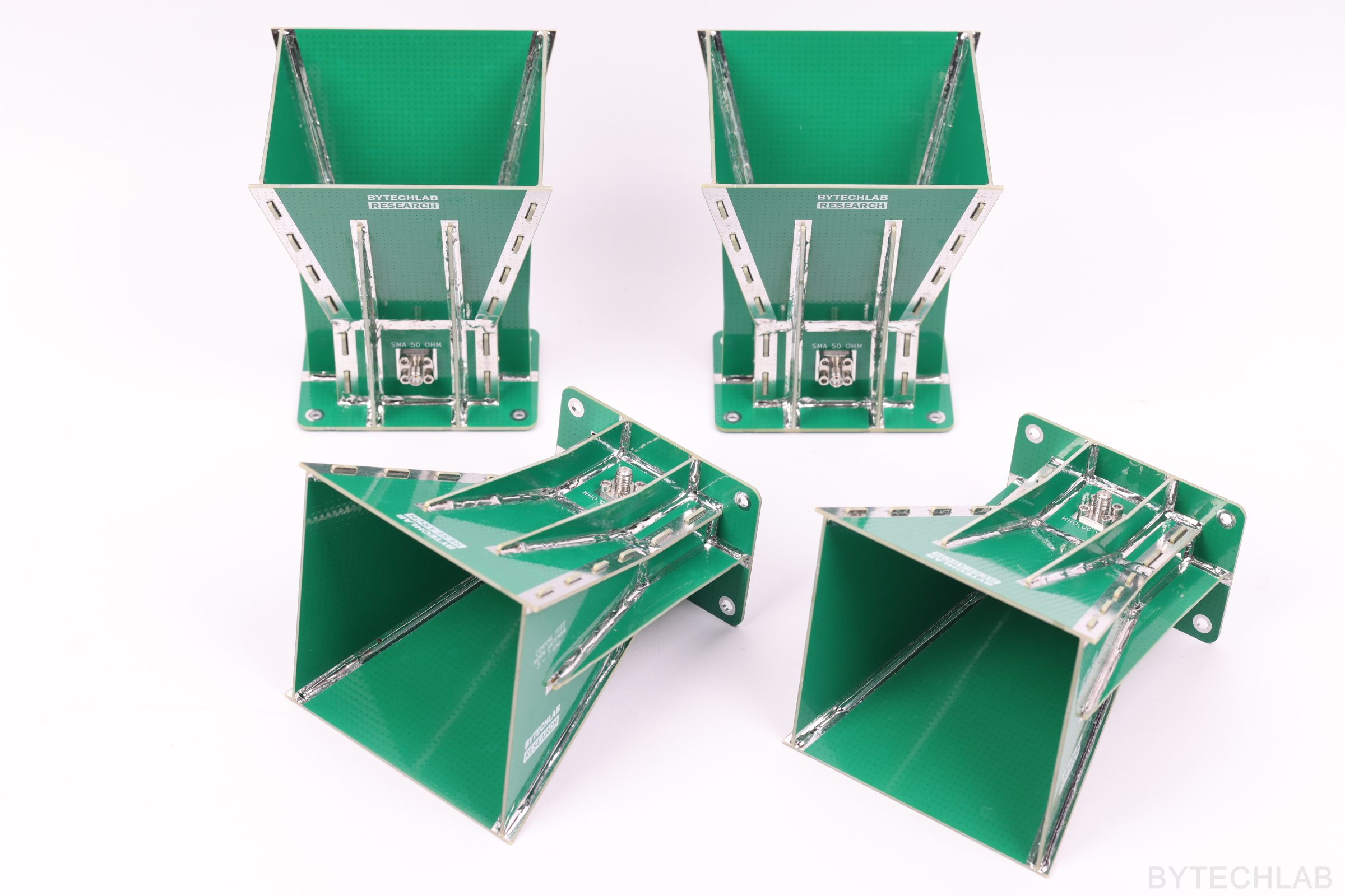
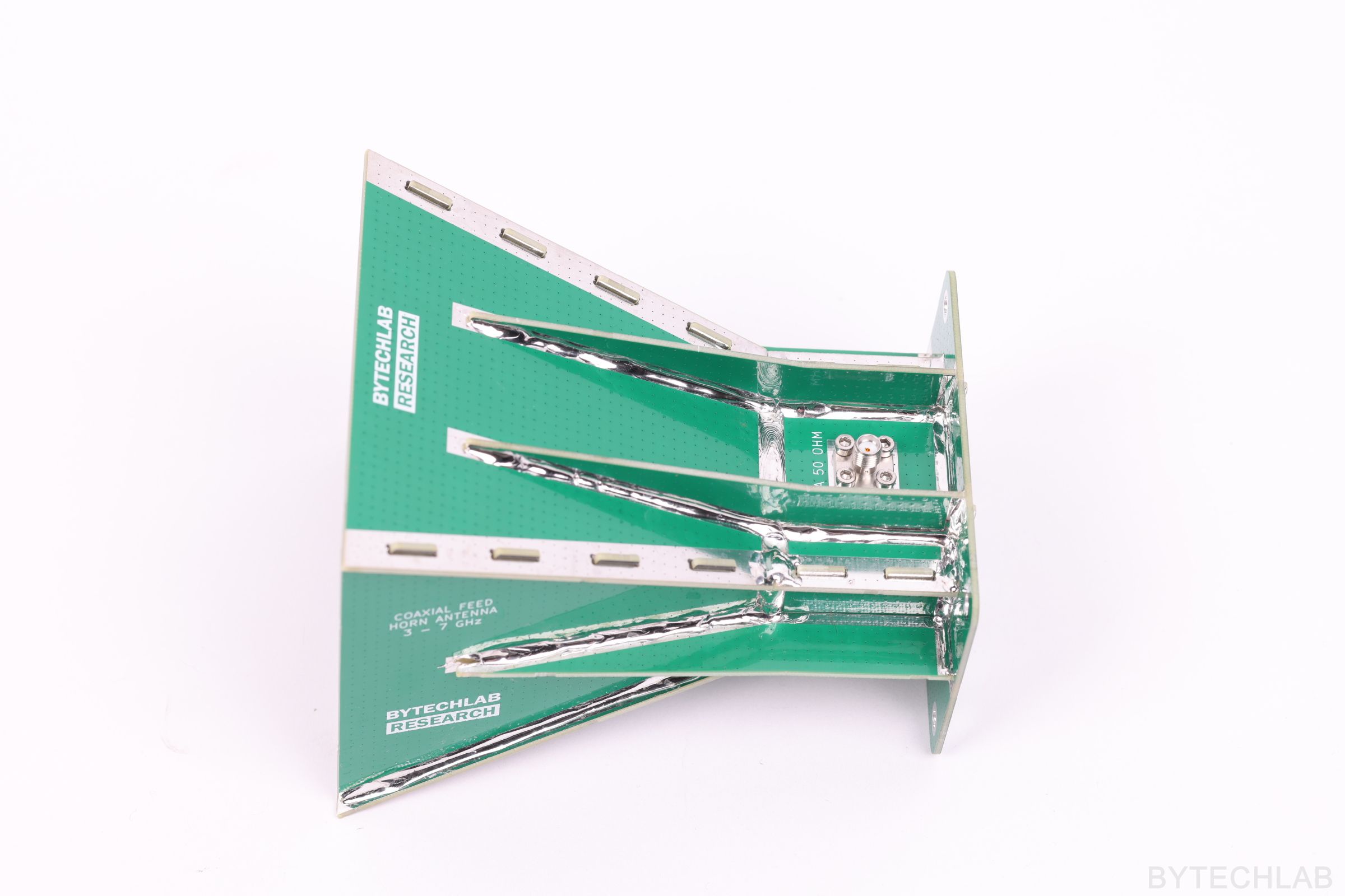
The antenna itself is quite simple, the most interesting part is the mechanical construction. The antenna consists of many 2-layer FR4 PCB’s with tabs and slots which are later soldered together to create mechanically stable construction. The solder also helps with the antenna performance (for example by sealing the gaps between the PCB’s to minimize fields leakage).

I’ll go through the principle of operation, the CST simulations, the build and the measurements, and finally check how the antenna behaves in a 6-element receive array for my radar project. One antenna costs about 15–20 USD and takes roughly one hour to assemble.

This yet another antenna that will be added to my open-source antenna library.

1) Research & Principle of operation & Simplified Parametric 3D-EM Simulations

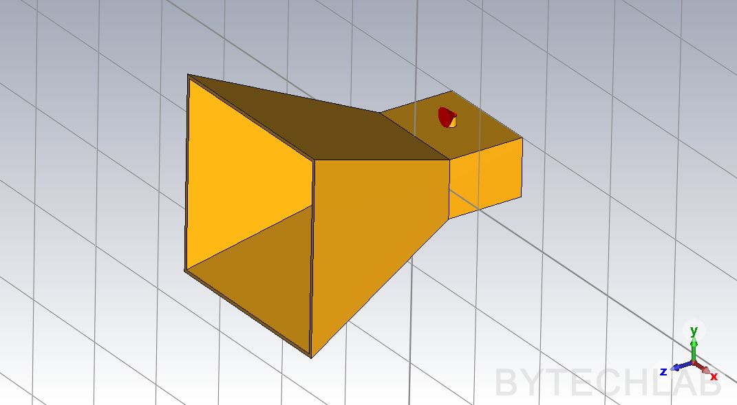
PCB Coaxial-Fed Horn Antenna (3-7 GHz) - Parametric simulation - 3D Model 2 — Parametric simulation – 3D Model 2

How does it work?

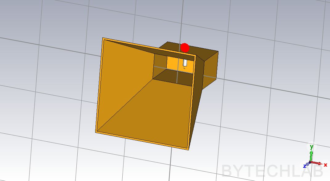
A pyramidal horn is basically a rectangular waveguide whose walls gradually open up in both directions. The flare works as a smooth transition between the waveguide and free space (an open waveguide end would reflect a lot of energy back), and the bigger aperture gives the antenna its gain. My antenna consists of three parts:

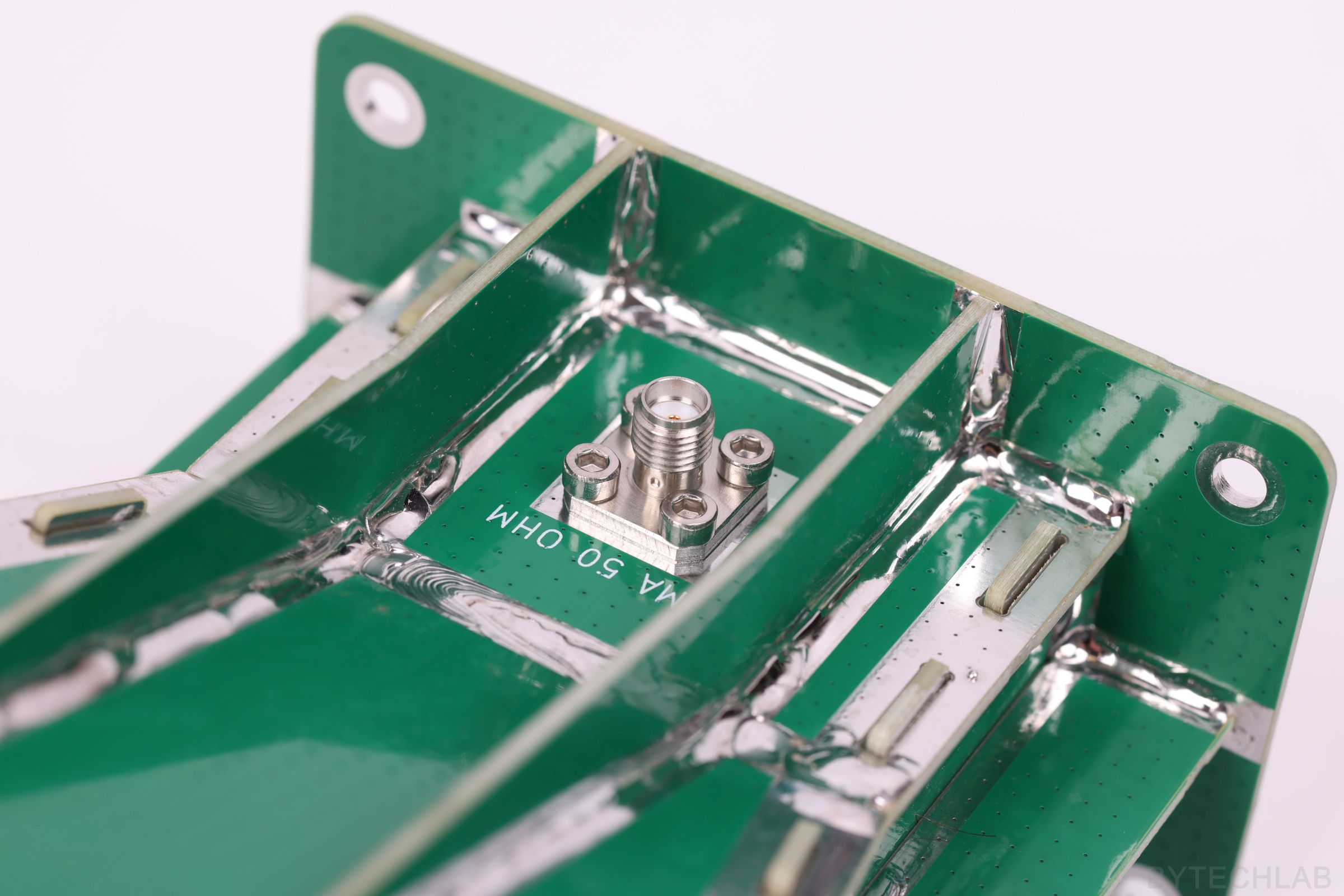
Coaxial probe – the pin of the SMA connector, together with its PTFE dielectric, sticks into the waveguide and works like a small monopole antenna [2], [4].
Waveguide section with a back wall – the wave radiated backwards by the probe reflects from the back wall. The distance between the probe and the wall decides whether this reflection helps or hurts the impedance match [2], [3].
Flare – guides the wave out and radiates it.

Antenna dimensions

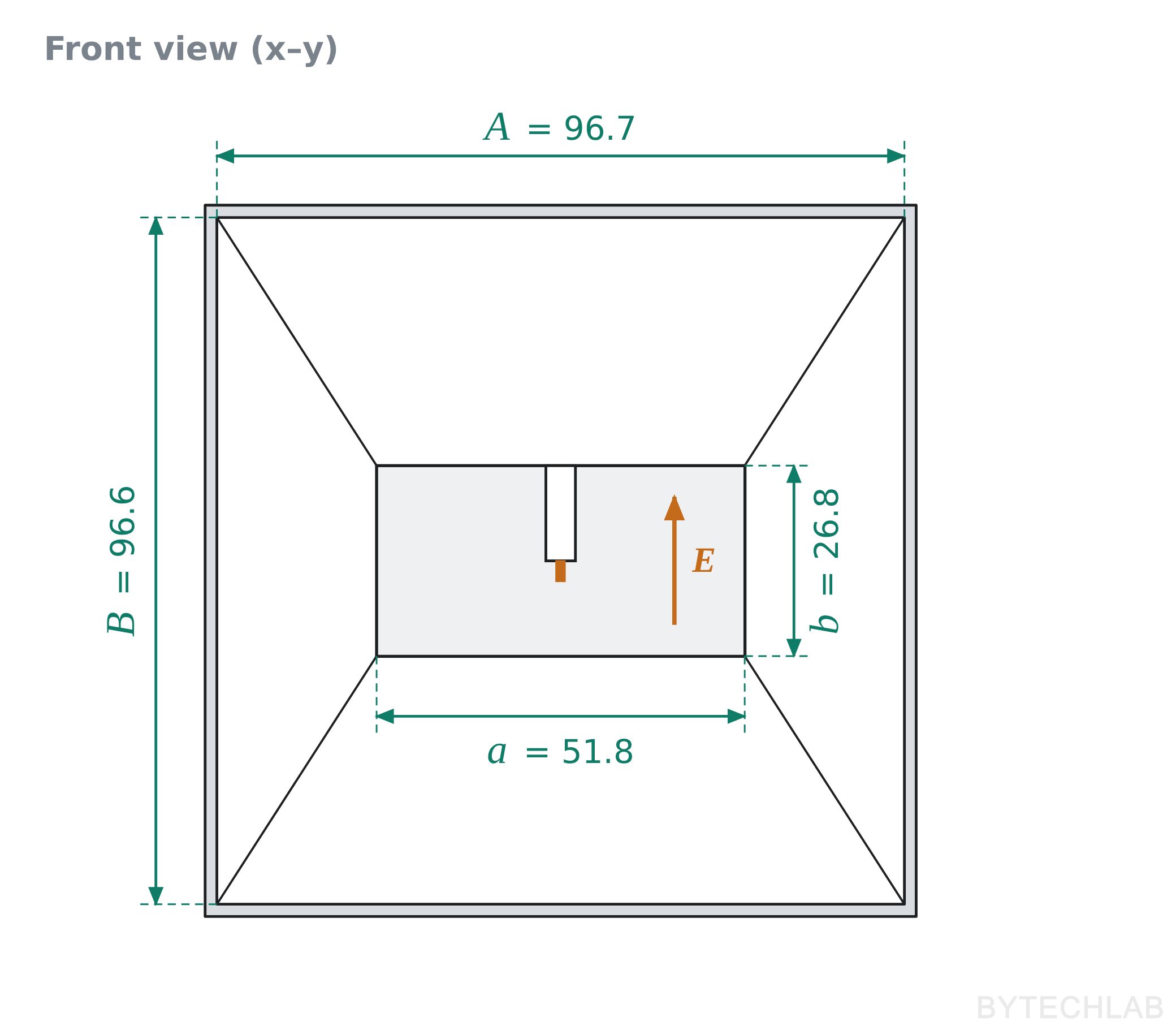
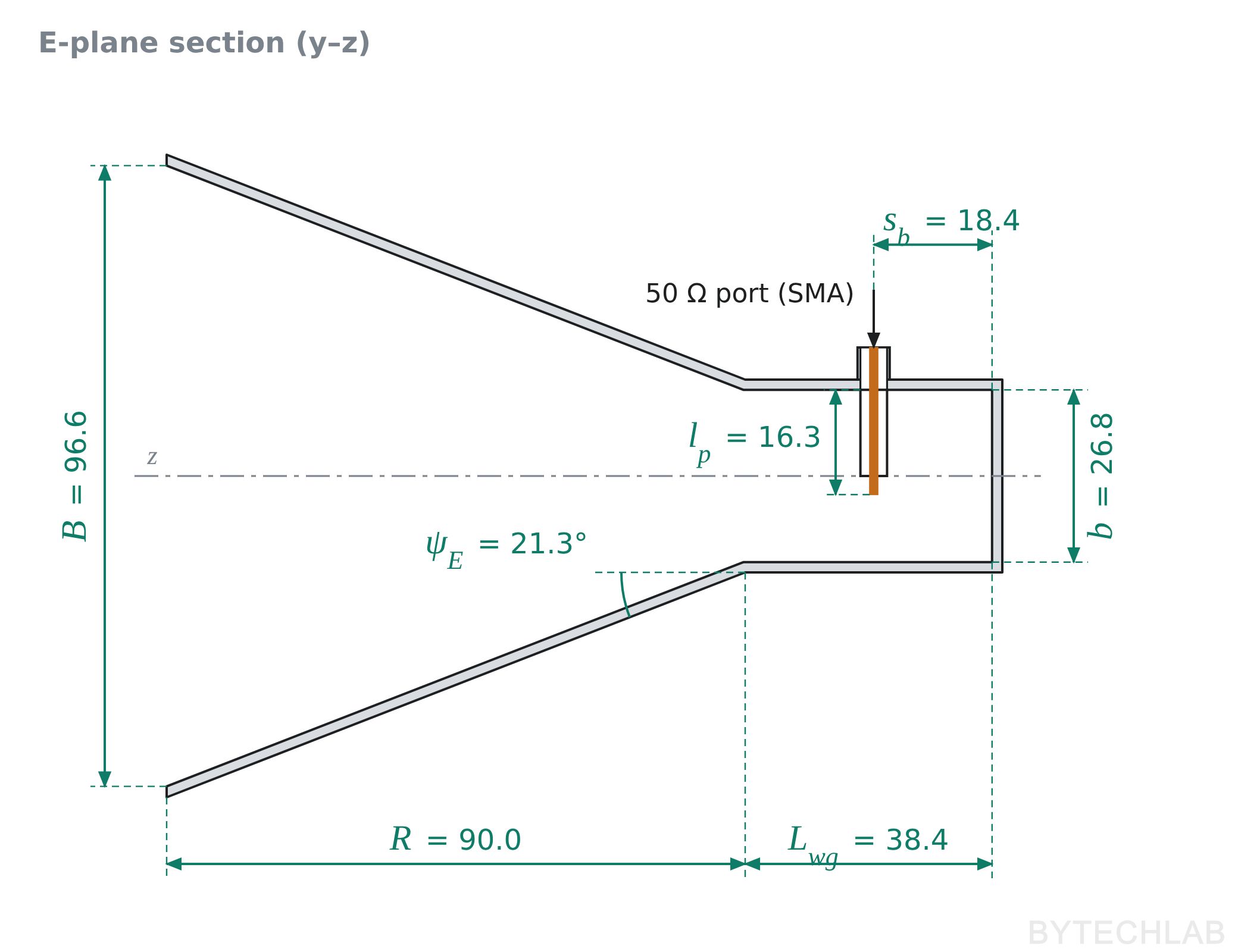
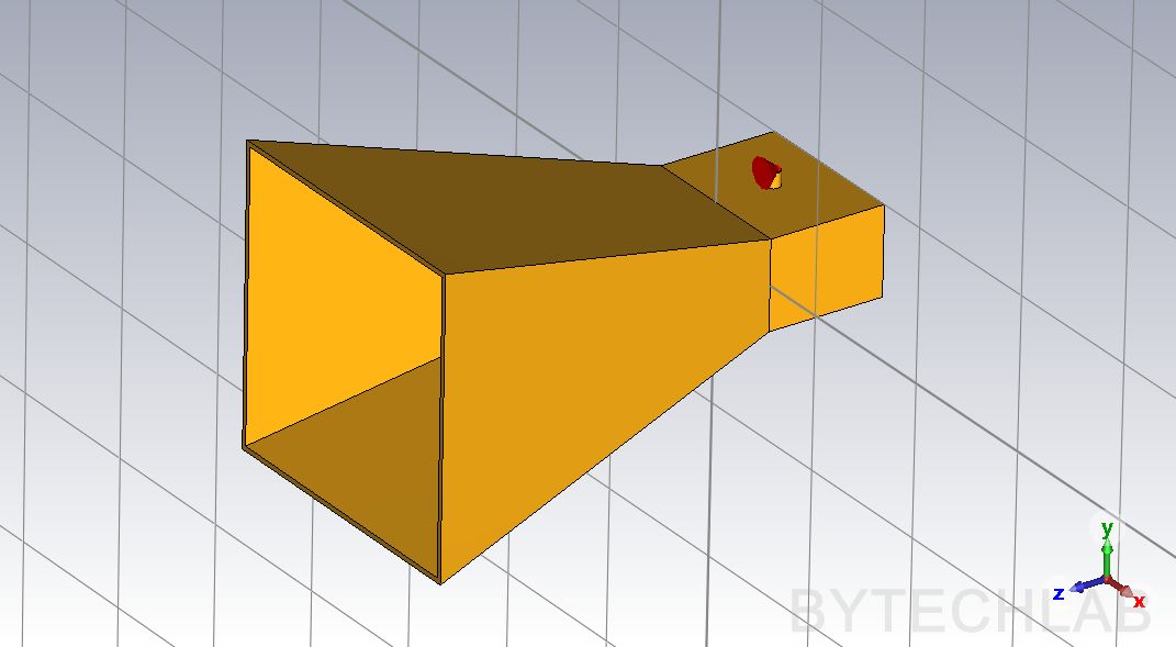
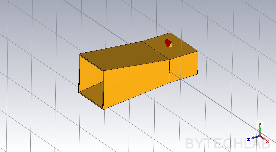
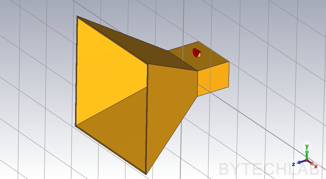
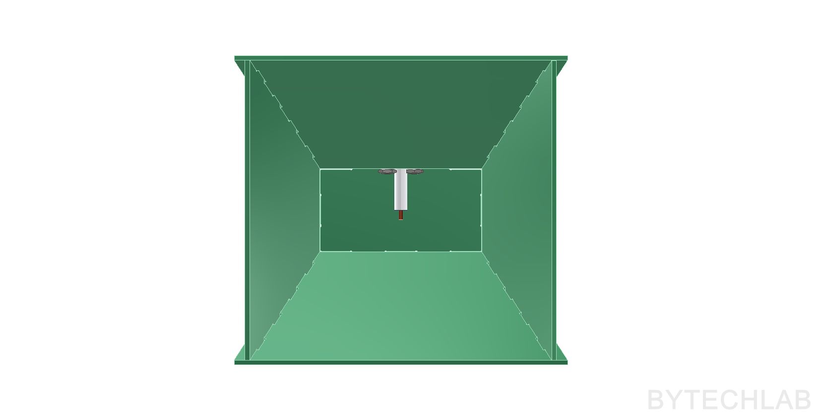
The drawings below show the simplified antenna (the CST model, without tabs and slots) with the names of the dimensions that I will use in the rest of the post. All dimension are shown between internal surfaces (the most important ones).

PCB Coaxial-Fed Horn Antenna (3-7 GHz) - Antenna Dimensions - E-plane — Antenna Dimensions – E-plane

PCB Coaxial-Fed Horn Antenna (3-7 GHz) - Antenna Dimensions - Probe Details — Antenna Dimensions – Probe Details

PCB Coaxial-Fed Horn Antenna (3-7 GHz) - Antenna Dimensions - H-plane — Antenna Dimensions – H-plane

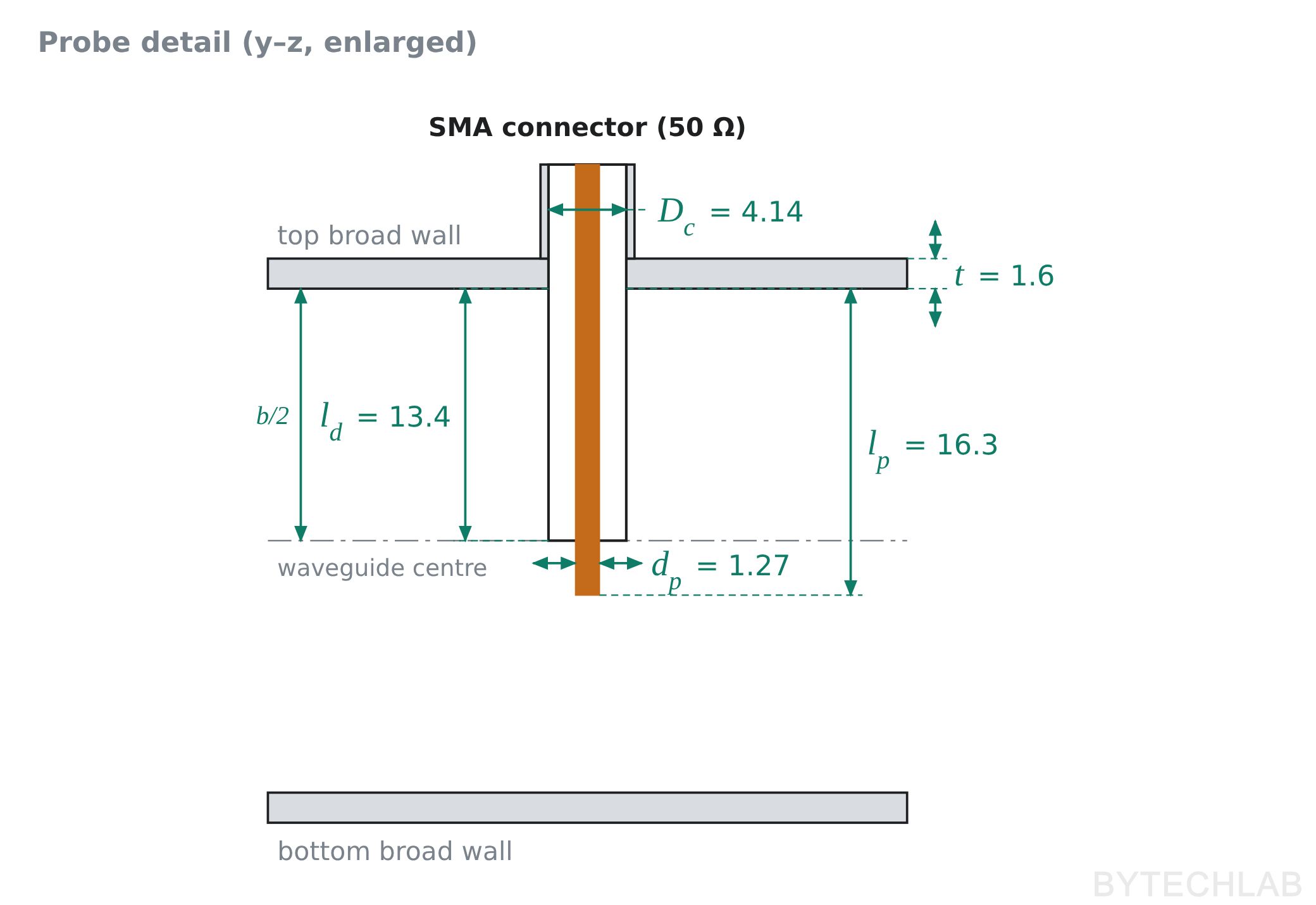
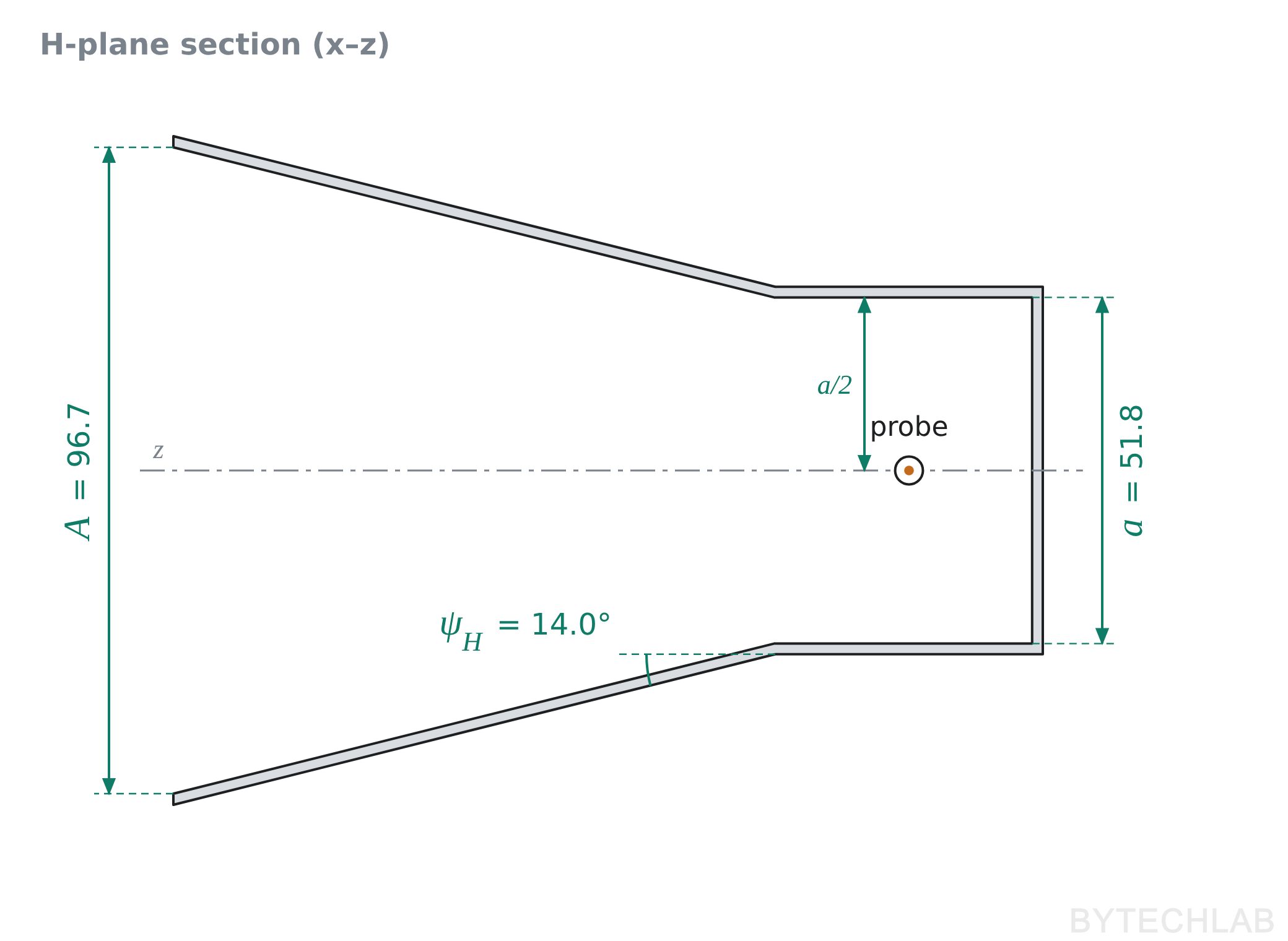
Symbol	Dimension	[mm]
a × b	Waveguide (inner)	51.8 × 26.8
s_b	Probe → back wall	18.4
l_p	Probe length	16.3
d_p / D_c	Pin / PTFE diameter	1.27 / 4.14
R	Flare length	90.0
A × B	Aperture (inner)	96.7 × 96.6

The probe dimensions come straight from the connector (Amphenol 901-2PF705590AM): its PTFE dielectric sticks out 15.0 mm from the flange, so after passing the 1.6 mm PCB wall 13.4 mm of it ends up inside the waveguide, followed by 2.9 mm of bare pin [8].

Waveguide modes – what sets the frequency range

Before going further, it’s worth looking at what actually happens inside the waveguide section, because it explains both the lower and the upper frequency limit of this antenna.

A waveguide is simply a metal pipe that carries electromagnetic waves. A wave inside it can’t travel freely like in open space, because the electric field along the metal walls has to be zero – the metal shorts it out. The only field shapes that survive are the ones that “fit” between the walls: a whole number of half-waves across the width and across the height. Each of these allowed shapes is called a mode. Across the pipe the field forms a standing pattern, along the pipe it travels.

The name tells you the shape. In TE_mn or TM_mn, m is the number of half-waves across the wide side a and n across the narrow side b. TE (transverse electric) means the E-field lies entirely in the cross-section, TM (transverse magnetic) means the same for the magnetic field. My antenna uses the simplest one, TE₁₀: one half-wave across a, strongest in the middle and zero at the side walls, and constant from top to bottom. You can explore the first eight modes of my waveguide below. Please note that not all of the modes are excited by the probe.

Lower frequency limit – the cutoff

A mode can only exist if its half-waves fit across the pipe. For TE₁₀, half a wavelength has to fit across a; at low frequencies the wavelength is simply too long. A nice way to picture this: TE₁₀ are ordinary plane waves bouncing between the side walls in a zig-zag. This isn’t just a cartoon – mathematically the TE₁₀ field is exactly the sum of two such plane waves, with the metal walls working as mirrors (a bit like the core of an optical fibre) [6]. The lower the frequency, the steeper the bounce, and at the cutoff frequency the waves bounce straight across and don’t move forward at all:

\begin{array}{c} f_{c} = \frac{c}{2a} = \frac{299.79\cdot 10^{6}\ \mathrm{m/s}}{2 \cdot 51.8\ \mathrm{mm}} \approx 2.89\ \mathrm{GHz} \qquad (1) \\ \scriptstyle \text{Source: [3] eq. (2); [6] eq. (3.85)} \end{array}

Pozar [6] writes the cutoff for a waveguide filled with any material. My waveguide is filled with air, where 1/√(μ₀ε₀) is simply the speed of light c.

\begin{array}{c} \begin{aligned} f_{c,10} &= \frac{1}{2a\sqrt{\mu\varepsilon}} && \text{[6] eq. (3.85)} \\ \frac{1}{\sqrt{\mu_0\varepsilon_0}} &= c && \text{the waveguide is filled with air} \\ \Rightarrow\ f_{c} &= \frac{c}{2a} && \end{aligned} \\ \scriptstyle \text{Derivation of eq. (1)} \end{array}

Below this frequency the energy is simply reflected back to the connector – you can see it in all S₁₁ plots: 0 dB up to ~2.5 GHz, then a steep drop to below −10 dB at ~3 GHz. The drop starts a bit below the cutoff because my waveguide section is very short: below cutoff the field doesn’t travel but decays. This is also why the realized gain at 1–2 GHz is so negative – the antenna doesn’t radiate there at all.

Guided wavelength

Because the wave zig-zags, its pattern along the pipe repeats over a longer distance than in free space – the guided wavelength is [3], [6]:

\begin{array}{c} \lambda_g = \frac{\lambda_0}{\sqrt{1 – \left(\frac{f_{c}}{f}\right)^{2}}} \qquad (2) \\ \scriptstyle \text{Source: [3] eq. (12); [4] eq. (9); [6] eq. (3.87)} \end{array}

[3] writes the guided wavelength with λ₀/2a. Replacing λ₀ with c/f and using eq. (1) turns this into the frequency ratio f_c/f, which shows directly what happens close to the cutoff.

\begin{array}{c} \begin{aligned} \lambda_g &= \frac{\lambda_0}{\sqrt{1-\left(\lambda_0/2a\right)^{2}}} && \text{[3] eq. (12)} \\ \frac{\lambda_0}{2a} &= \frac{c/f}{2a} = \frac{c/2a}{f} = \frac{f_c}{f} && \text{using } \lambda_0 = c/f \text{ and eq. (1)} \\ \Rightarrow\ \lambda_g &= \frac{\lambda_0}{\sqrt{1-\left(f_c/f\right)^{2}}} && \end{aligned} \\ \scriptstyle \text{Derivation of eq. (2)} \end{array}

Close to the cutoff it grows enormously: in my antenna λ_g changes from ~379 mm at 3 GHz to ~47 mm at 7 GHz. Below the cutoff the wave stops travelling altogether – the field just oscillates in place and dies away from the probe.

Upper frequency limit – higher-order modes

Every mode has its own cutoff, so at higher frequencies the waveguide can also carry other modes besides TE₁₀. Whether they actually appear depends on the probe: it’s a small antenna pointing in the vertical direction, so it can only excite a mode that has a vertical E-field where the probe is [6]:

TE₀₁ (5.59 GHz) – its field is horizontal, perpendicular to the probe. Not excited.
TE₂₀ (5.79 GHz) – zero field in the middle, exactly where the probe is. Not excited.
TE₁₁ / TM₁₁ (6.30 GHz) – the vertical field changes sign between the top and bottom half. A probe spanning the full height would cancel it out, but mine ends just 2.9 mm below the centre. Excited.

So from ~6.3 GHz the probe starts exciting unwanted modes, which degrade the matching and later the beam. This agrees nicely with the simulations, where |S₁₁| rises above −10 dB just above 6 GHz.

Feeding the waveguide – probe and back wall

With λ_g changing so much across the band, matching the probe is the tricky part of this design. The classic design rule for a coax-to-waveguide transition is a quarter-wave probe and a quarter-wave distance to the back wall [3], [4]:

\begin{array}{c} l_p \approx \frac{\lambda_0}{4}, \qquad s_b \approx \frac{\lambda_g}{4} \qquad (3) \\ \scriptstyle \text{Source: [3] eq. (13); [4] eq. (10)} \end{array}

My back wall distance s_b = 18.4 mm is exactly λ_g/4 at 5.0 GHz – right in the middle of the band. The probe (16.3 mm) would be a quarter-wave at 4.6 GHz if it were a bare pin in air. A dielectric sleeve around a monopole lowers its resonant frequency – it makes it electrically longer [1] – so with the PTFE around it my probe resonates somewhat lower. The catch is that these rules are only correct at one frequency, so they can only be a starting points. That’s why I tuned the final values in the simulations. A thicker metal probe also gives a wider bandwidth [2], [4] – in my case the pin diameter is simply fixed by the SMA connector. And the connector itself stays close to 50 Ω all the way into the waveguide (48.9 Ω from its dimensions [4], [6]).

Gain

The gain of a horn depends on its aperture A × B and the aperture efficiency ε_ap [1], [2]:

\begin{array}{c} G = \frac{4\pi\,\varepsilon_{ap}\,A\,B}{\lambda_0^{2}} \qquad (4) \\ \scriptstyle \text{Source: [1] eq. (13-53); [2] eq. (1); [3] eq. (14); [5] eq. (1)} \end{array}

The efficiency is never 100%: the field is weaker towards the side walls, and in a short horn the wave reaches the edges of the aperture a bit later than the center, so the aperture isn’t illuminated in phase [2]. The higher the frequency, the bigger this phase error and the lower the efficiency. I calculated the expected directivity of my horn with the classic formula from Balanis [1], which takes both effects into account, and compared it with CST:

f [GHz]	Theory [dBi]	CST [dBi]	Aperture efficiency
3	9.6	10.1	78%
4	12.0	12.5	76%
5	13.8	13.8	73%
6	15.2	15.1	70%

The simple theory is within 0.5 dB of the full 3D simulation, which is a nice confirmation that the model makes sense. For comparison, a classic “optimum gain” horn reaches only about 50% efficiency [1].

Parametric simulations

With all of this in mind I built a fully parametric model in CST Studio. All of the dimensions shown above can be changed. With use of parametric 3D model I can quickly iterate to check which parameter combination works best for my application. As an example below you can see a sweep of two parameters – horn length (75 / 90 mm) and horn opening height (85 / 100 mm, outer). I’m not going to show all of the sweeps that I have made because there’s simply too much results – the results below are shown as an example.

PCB Coaxial-Fed Horn Antenna (3-7 GHz) - Parametric simulation - Realized Gain (Phi =0, Theta=0) — Parametric simulation – Realized Gain (Phi =0, Theta=0)

PCB Coaxial-Fed Horn Antenna (3-7 GHz) - Parametric simulation - Directivity (Const phi = 90 deg, 7 GHz) — Parametric simulation – Directivity (Const phi = 90 deg, 7 GHz)

PCB Coaxial-Fed Horn Antenna (3-7 GHz) - Parametric simulation - Directivity (Const phi = 90 deg, 6 GHz) — Parametric simulation – Directivity (Const phi = 90 deg, 6 GHz)

PCB Coaxial-Fed Horn Antenna (3-7 GHz) - Parametric simulation - Directivity (Const phi = 90 deg, 5 GHz) — Parametric simulation – Directivity (Const phi = 90 deg, 5 GHz)

PCB Coaxial-Fed Horn Antenna (3-7 GHz) - Parametric simulation - Directivity (Const phi = 90 deg, 4 GHz) — Parametric simulation – Directivity (Const phi = 90 deg, 4 GHz)

PCB Coaxial-Fed Horn Antenna (3-7 GHz) - Parametric simulation - Directivity (Const phi = 90 deg, 3 GHz) — Parametric simulation – Directivity (Const phi = 90 deg, 3 GHz)

PCB Coaxial-Fed Horn Antenna (3-7 GHz) - Parametric simulation - Table with parameters — Parametric simulation – Table with parameters

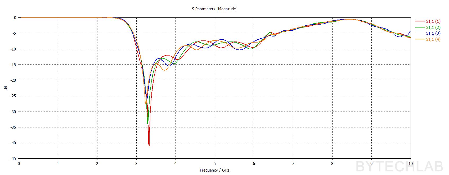
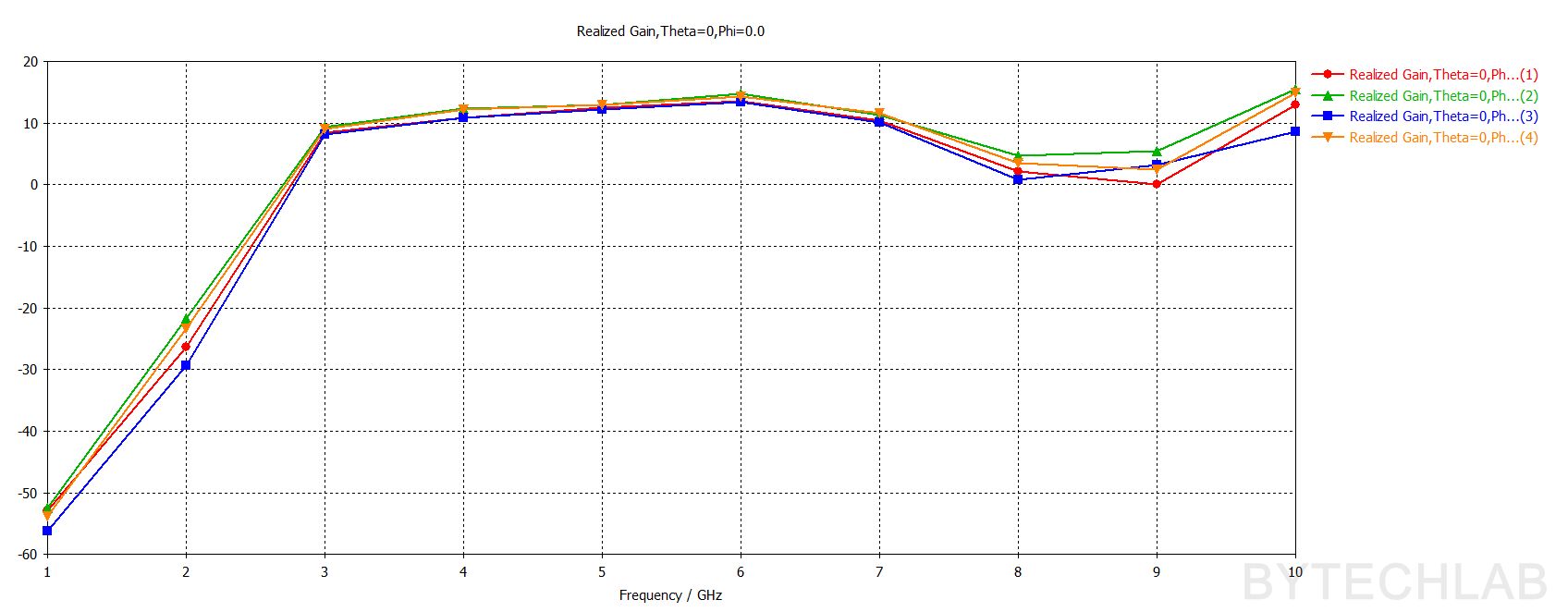
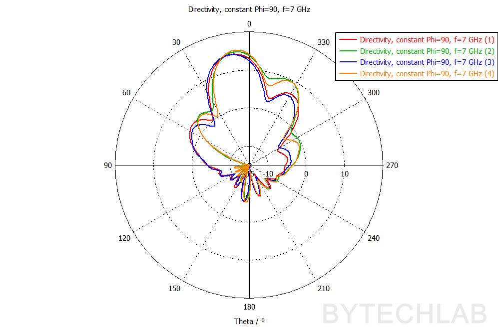
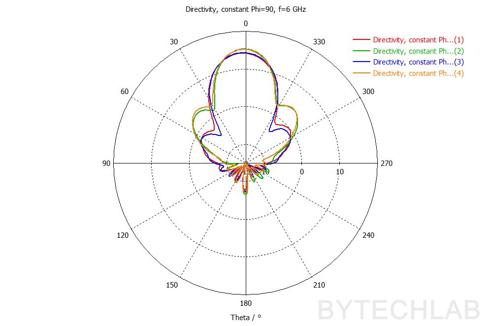
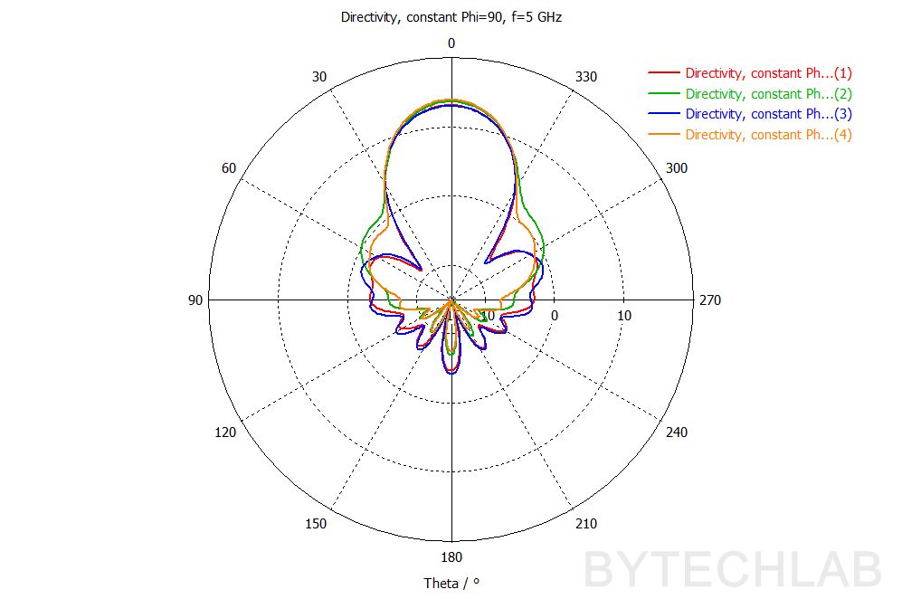
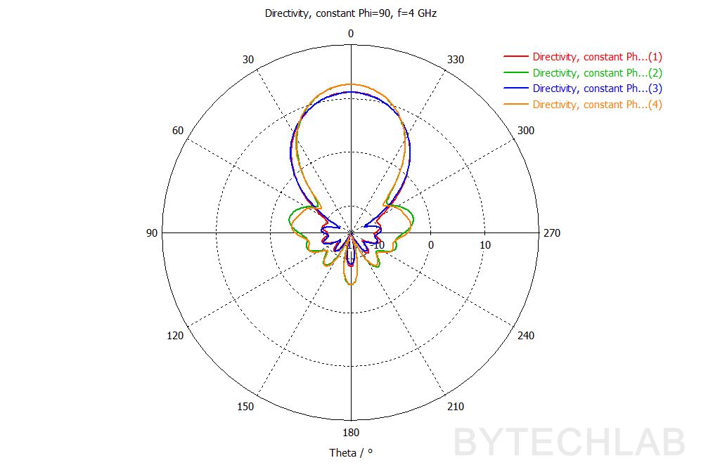
In the parametric simulation results above you can see that:

The lower band edge (~3 GHz) doesn’t move at all – it’s set by the waveguide cutoff, not by the horn.
All variants are best matched at ~3.3 GHz and stay below −10 dB up to ~4.2 GHz; above ~6.5 GHz the matching gets worse for all of them.
Realized gain is ~8–9.5 dBi at 3 GHz and ~13–14.5 dBi at 6 GHz, and it collapses at 8–9 GHz.

I chose run 4 (horn length 90 mm, opening height 100 mm) for the final design. After that I have exported this 3D model to Autodesk Inventor to add all of the necessary details and generate manufacturing documentation. After finalizing the MCAD design the 3D model will be once again exported, but this time the other way – From Inventor to CST just to sign off the final design.

PCB Coaxial-Fed Horn Antenna (3-7 GHz) - Parametric simulation - 3D Model 3 — Parametric simulation – 3D Model 3

PCB Coaxial-Fed Horn Antenna (3-7 GHz) - Parametric simulation - 3D Model 5 — Parametric simulation – 3D Model 5

PCB Coaxial-Fed Horn Antenna (3-7 GHz) - Parametric simulation - 3D Model 4 — Parametric simulation – 3D Model 4

PCB Coaxial-Fed Horn Antenna (3-7 GHz) - Parametric simulation - 3D Model 1 — Parametric simulation – 3D Model 1

2) MCAD & ECAD design

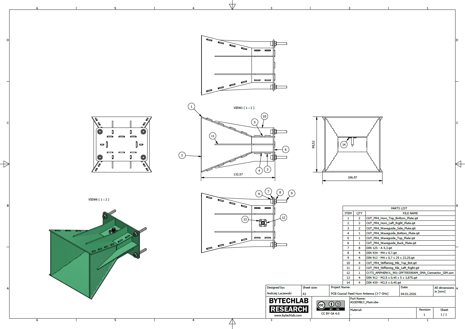
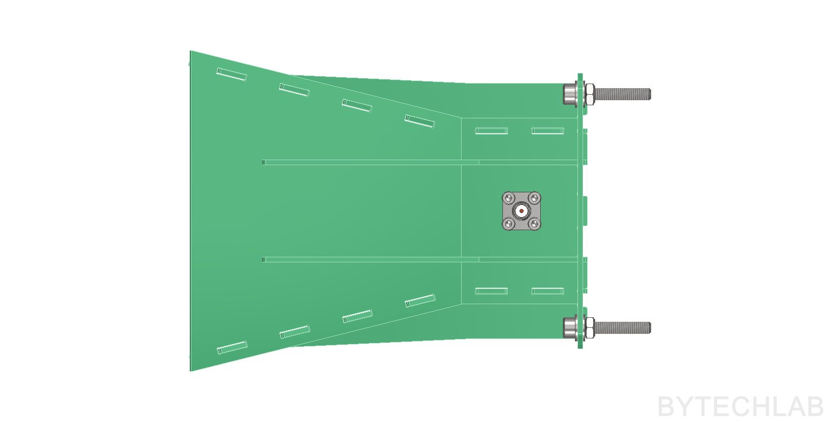
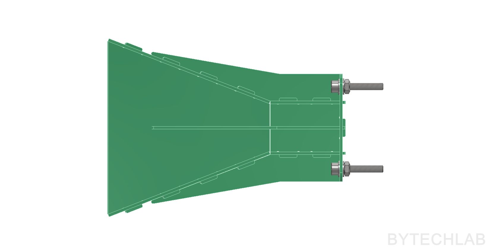
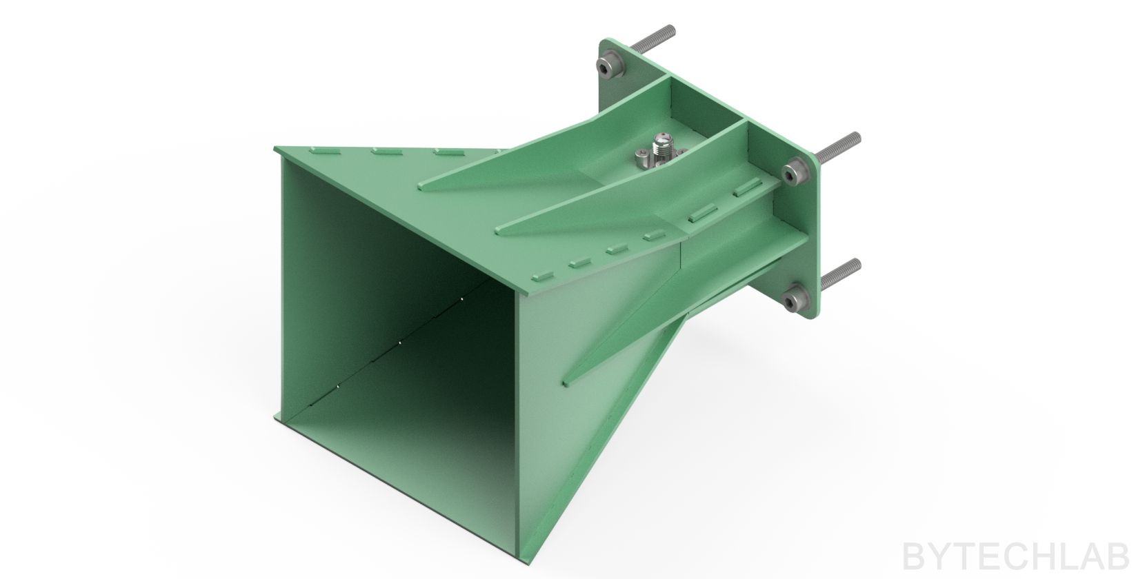
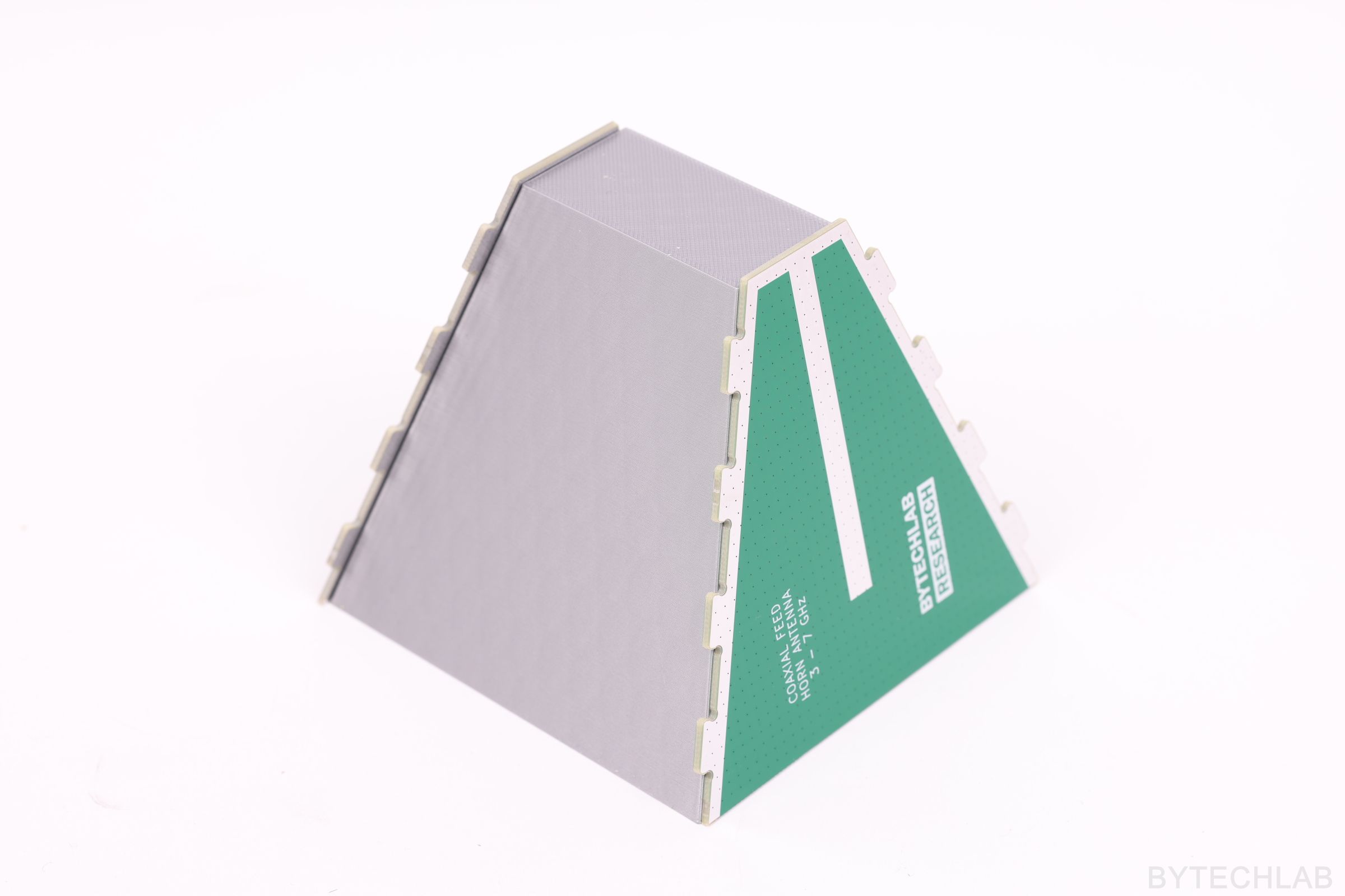
PCB Coaxial-Fed Horn Antenna (3-7 GHz) - MCAD - Drawing — MCAD – Drawing

Mechanically the antenna is just a set of 2-layer FR4 PCBs with tabs and slots that slot into each other and are then soldered together along all seams. The solder makes the structure rigid, but it also closes the gaps between the walls – an unsoldered seam would work as a slot antenna and leak energy. Only the inner copper layer matters electrically; the FR4 is just a carrier. Compared to sheet metal or 3D-printed and painted horns (like my double ridged horn), this gives solid copper walls, tight tolerances from the PCB fab and a very low price.

To make the antenna stiffer and more durable, I added reinforcing ribs to the outside of the horn walls: two on each of the wider top and bottom walls, and a single one on each side wall. They don’t affect the RF performance, because only the inner copper surface of the horn matters electrically.

To assemble the whole antenna you simply need to:

Order PCBs from JLCPCB (or any other PCB fab),
3D print the assembly jig,
Put the PCBs together on the jig and solder all seams,
Mount the SMA connector to the waveguide top plate with use of four screws and nuts.

In the GitHub repository (MCAD folder) you can find the following files:

Autodesk Inventor project of PCB Coaxial-Fed Horn Antenna,
Exported STL files for 3D printing,
Exported STEP file of the whole assembly,
Exported PDF file with assembly drawing, BOM and assembly instructions,
Exported assembly renders,

In the GitHub repository (ECAD folder) you can find the following files:

KiCAD projects of the PCB Coaxial-Fed Horn Antenna panels/parts,
Exported GERBER files for manufacturing,
Exported STEP file of the PCB’s,
Exported PDF file with schematics and layout,

PCB Coaxial-Fed Horn Antenna (3-7 GHz) - MCAD - Render - Top — MCAD – Render – Top

PCB Coaxial-Fed Horn Antenna (3-7 GHz) - MCAD - Render - Side — MCAD – Render – Side

PCB Coaxial-Fed Horn Antenna (3-7 GHz) - MCAD - Render - Realistic — MCAD – Render – Realistic

PCB Coaxial-Fed Horn Antenna (3-7 GHz) - MCAD - Render - Front — MCAD – Render – Front

3) Final EM simulation

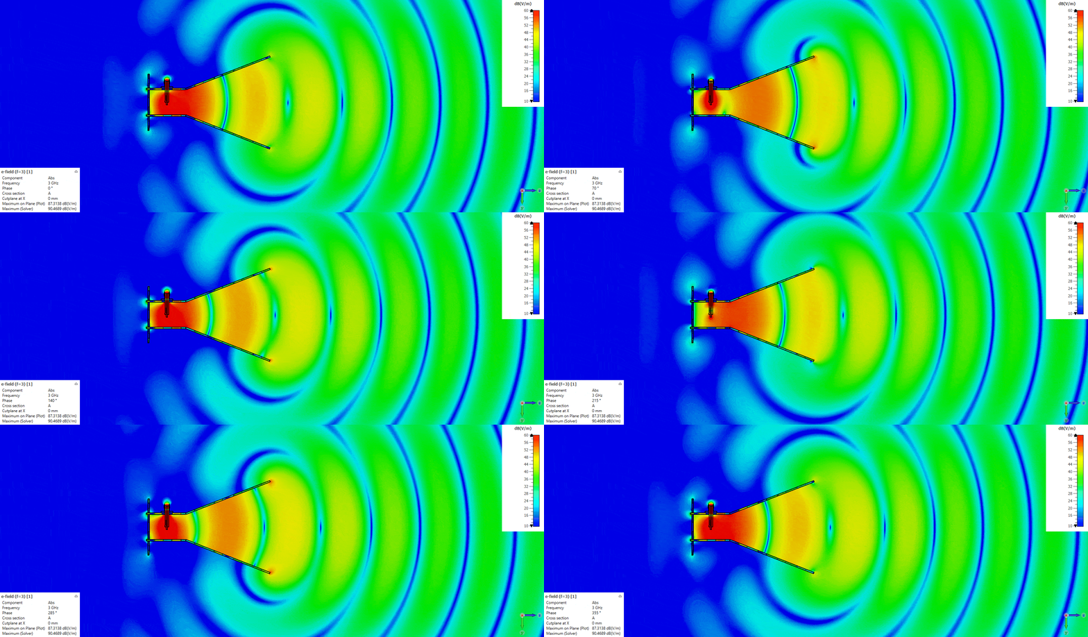
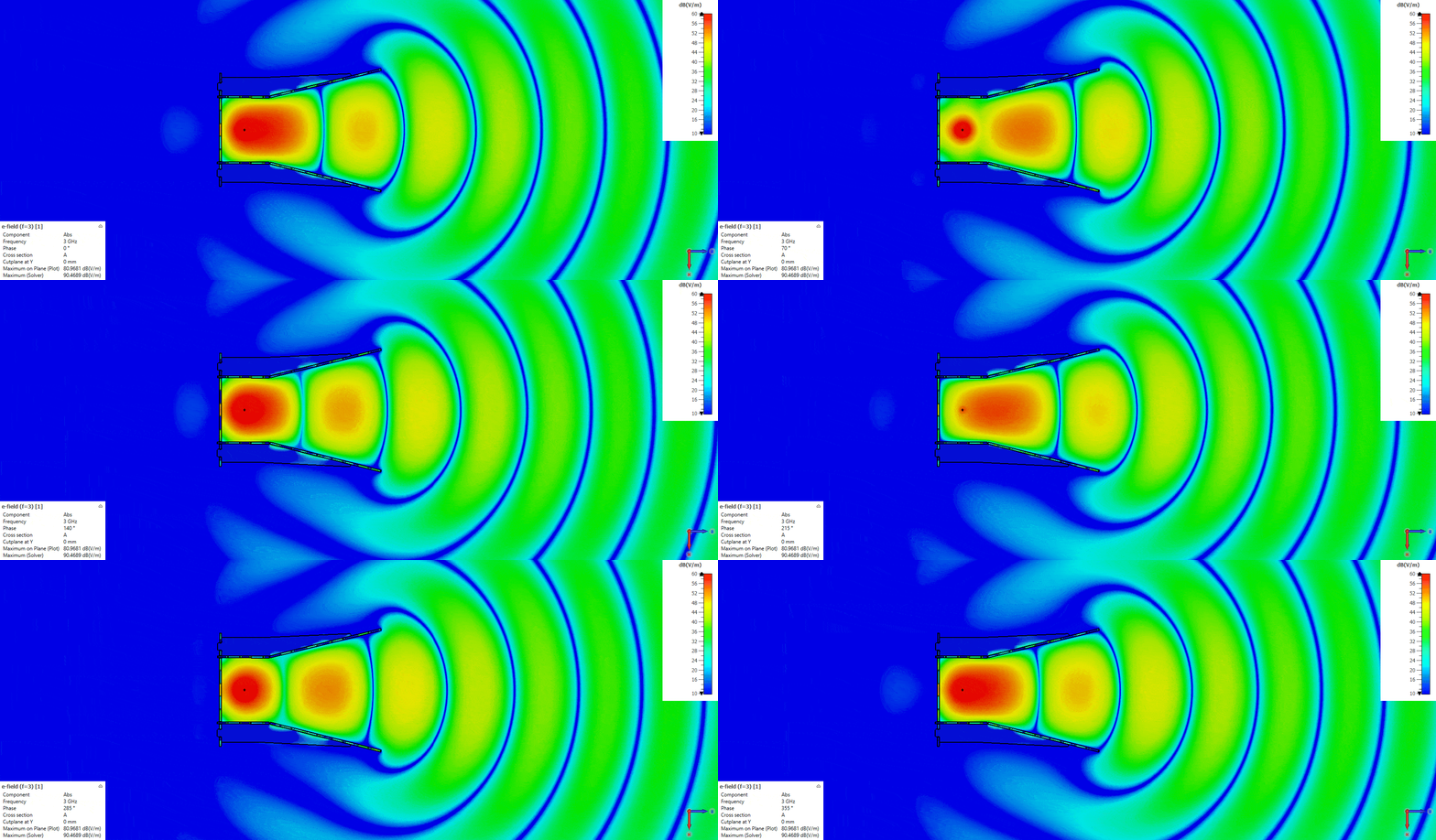
PCB Coaxial-Fed Horn Antenna (3-7 GHz) - Final simulation – Animated E field (3 GHz) – Section A — Final simulation – Animated E field (3 GHz) – Section A

PCB Coaxial-Fed Horn Antenna (3-7 GHz) - Final simulation – Animated E field (3 GHz) – Section B — Final simulation – Animated E field (3 GHz) – Section B

As described before the final 3D model from Autodesk Inventor was imported back to CST to perform final checks. Some of the geometry had to be simplified in order to reduce mesh size (for example there are no solder joints), because of this on the animations you can see the E field leaking from the gaps between the PCB’s. This is not going to be a issue in a real antenna, for this simulation it is good enough (it only will affect the side / back lobes).

The animations also show the wave launched by the probe travelling through the horn. Notice how the distance between the field maxima inside the horn changes with frequency: at 3 GHz, just above the cutoff, the wavelength in the waveguide is very long and the whole waveguide is filled with practically one maximum, while at 5 and 7 GHz several of them fit inside.

PCB Coaxial-Fed Horn Antenna (3-7 GHz) - Final simulation – Animated E field (5 GHz) – Section A — Final simulation – Animated E field (5 GHz) – Section A

PCB Coaxial-Fed Horn Antenna (3-7 GHz) - Final simulation – Animated E field (5 GHz) – Section B — Final simulation – Animated E field (5 GHz) – Section B

PCB Coaxial-Fed Horn Antenna (3-7 GHz) - Final simulation – Animated E field (7 GHz) – Section A — Final simulation – Animated E field (7 GHz) – Section A

PCB Coaxial-Fed Horn Antenna (3-7 GHz) - Final simulation – Animated E field (7 GHz) – Section B — Final simulation – Animated E field (7 GHz) – Section B

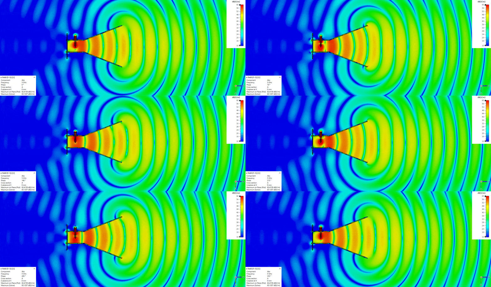
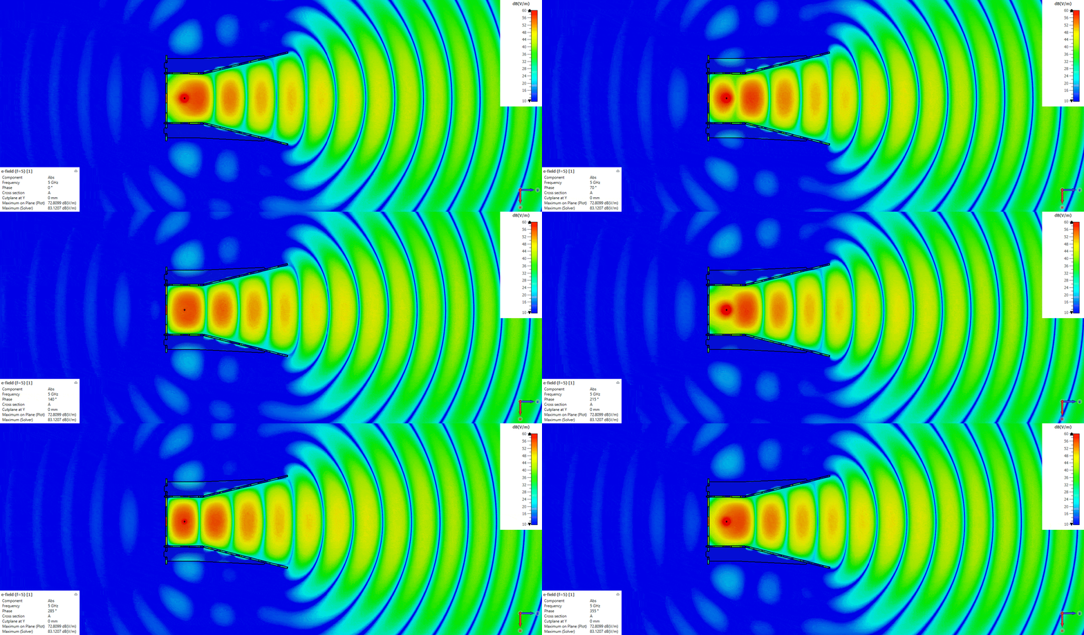
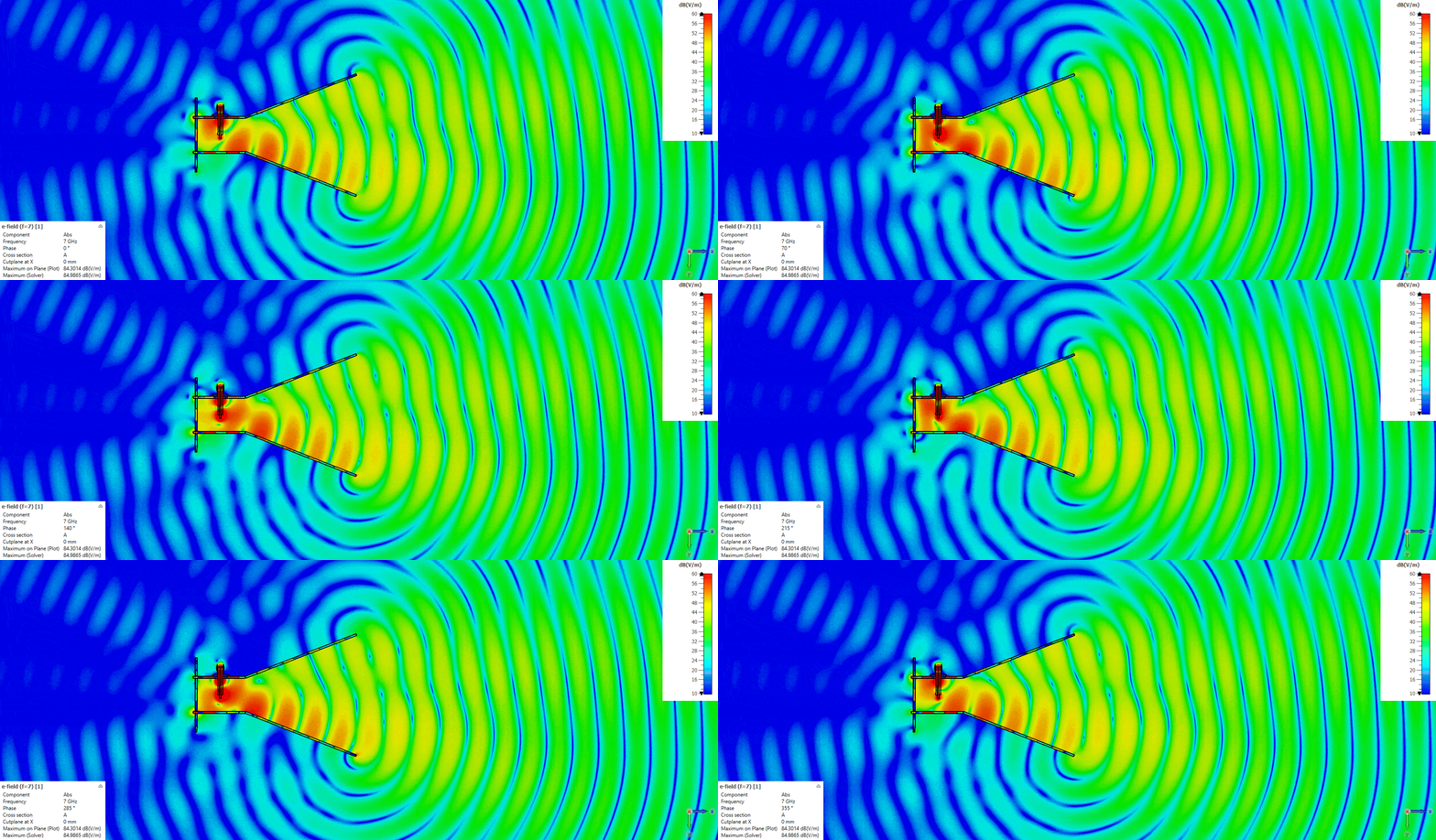
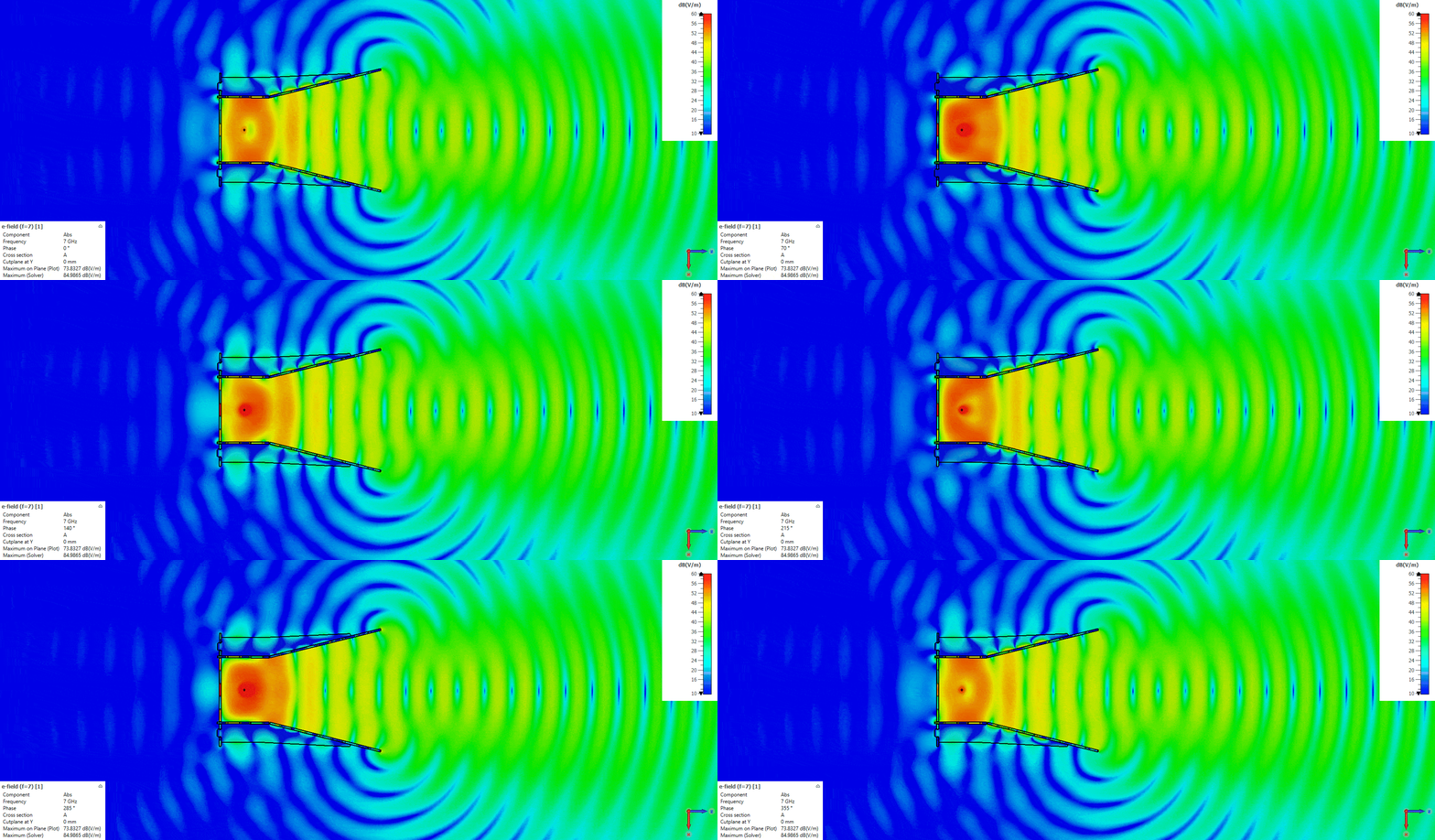
In the 3D directivity plots the beam gets narrower with increasing frequency, as expected. At 2 GHz the antenna is below cutoff (the efficiency is very low as expected), and from 8 GHz up the beam breaks into several lobes because of the higher-order modes.

PCB Coaxial-Fed Horn Antenna (3-7 GHz) - Final simulation – Directivity 3D (2 GHz) — Final simulation – Directivity 3D (2 GHz)

PCB Coaxial-Fed Horn Antenna (3-7 GHz) - Final simulation – Directivity 3D (3 GHz) — Final simulation – Directivity 3D (3 GHz)

PCB Coaxial-Fed Horn Antenna (3-7 GHz) - Final simulation – Directivity 3D (4 GHz) — Final simulation – Directivity 3D (4 GHz)

PCB Coaxial-Fed Horn Antenna (3-7 GHz) - Final simulation – Directivity 3D (5 GHz) — Final simulation – Directivity 3D (5 GHz)

PCB Coaxial-Fed Horn Antenna (3-7 GHz) - Final simulation – Directivity 3D (6 GHz) — Final simulation – Directivity 3D (6 GHz)

PCB Coaxial-Fed Horn Antenna (3-7 GHz) - Final simulation – Directivity 3D (7 GHz) — Final simulation – Directivity 3D (7 GHz)

PCB Coaxial-Fed Horn Antenna (3-7 GHz) - Final simulation – Directivity 3D (8 GHz) — Final simulation – Directivity 3D (8 GHz)

PCB Coaxial-Fed Horn Antenna (3-7 GHz) - Final simulation – Directivity 3D (9 GHz) — Final simulation – Directivity 3D (9 GHz)

PCB Coaxial-Fed Horn Antenna (3-7 GHz) - Final simulation – Directivity 3D (10 GHz) — Final simulation – Directivity 3D (10 GHz)

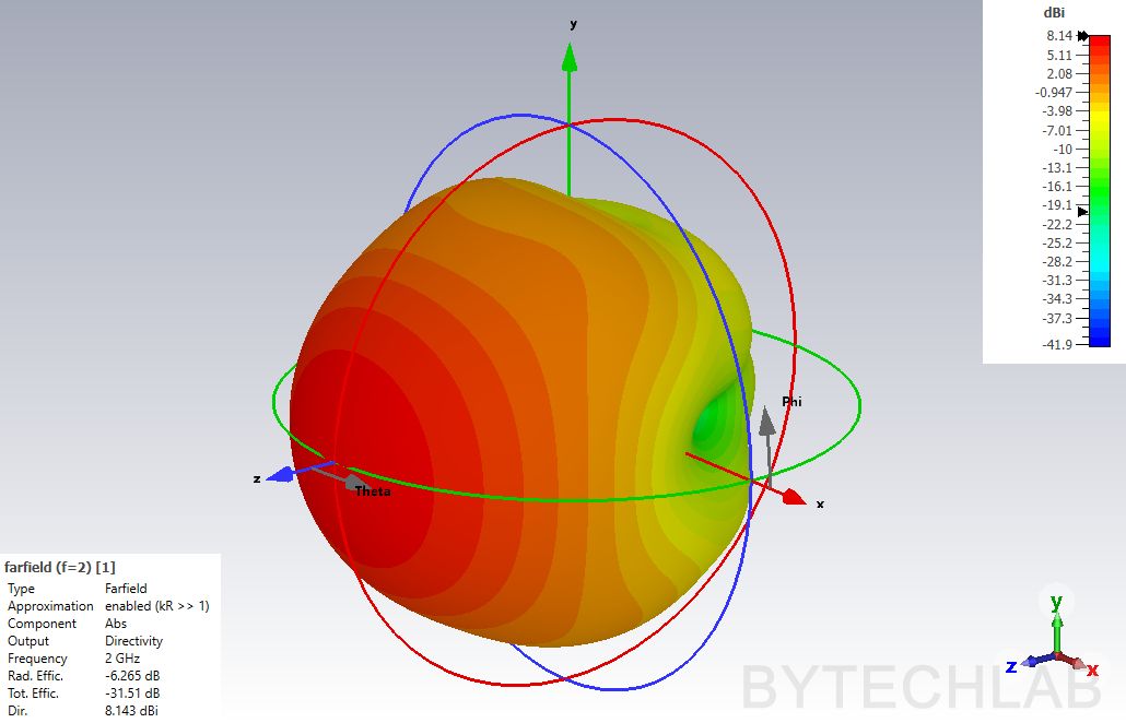
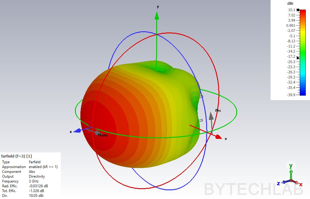
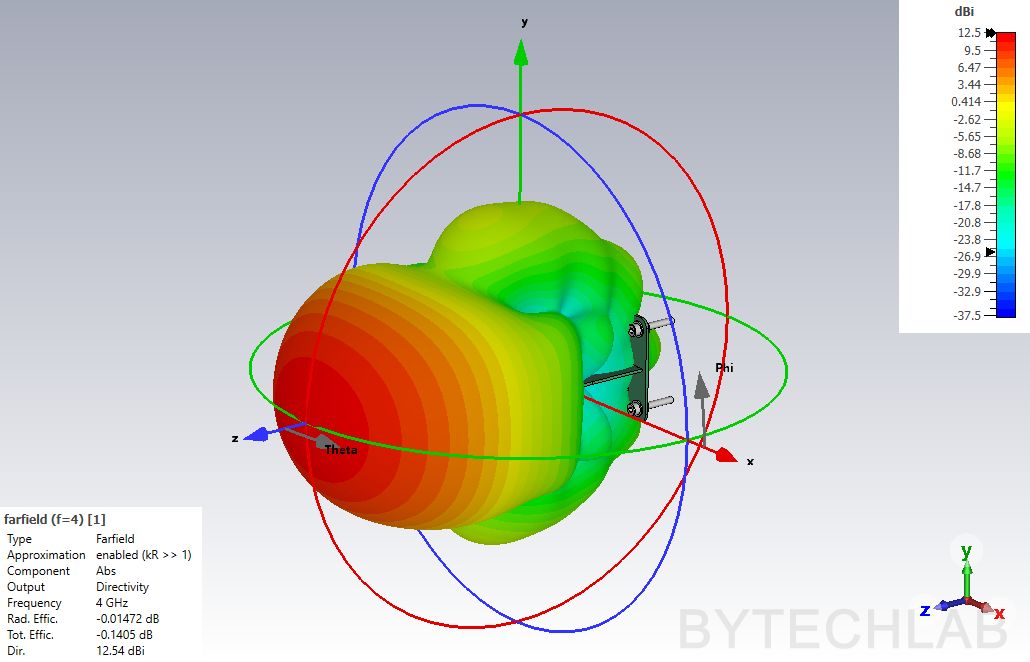
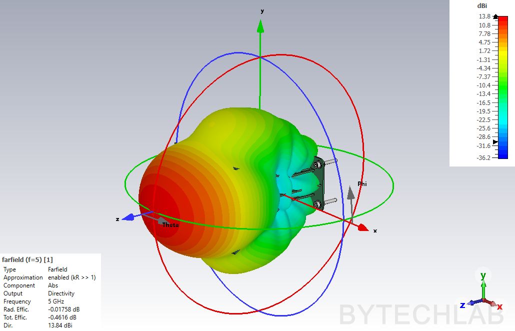
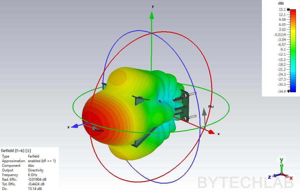
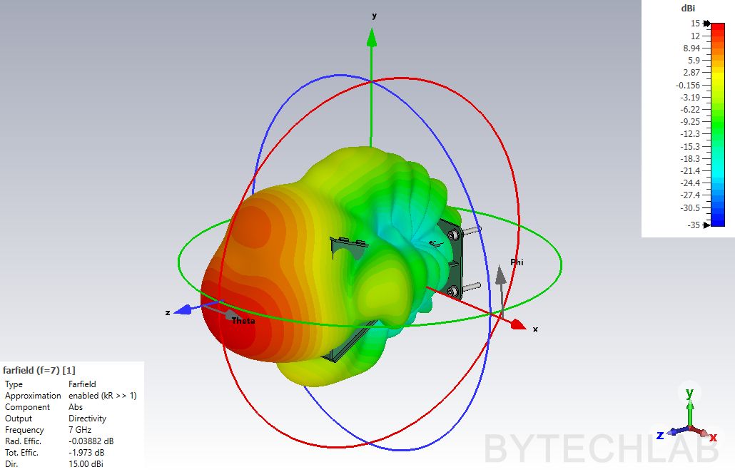
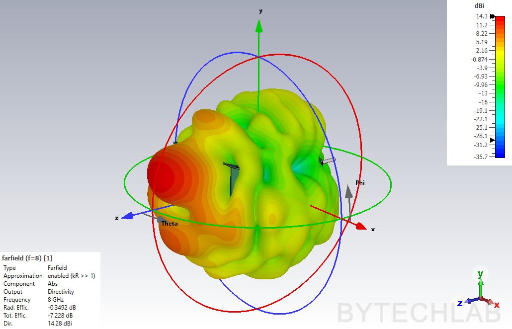
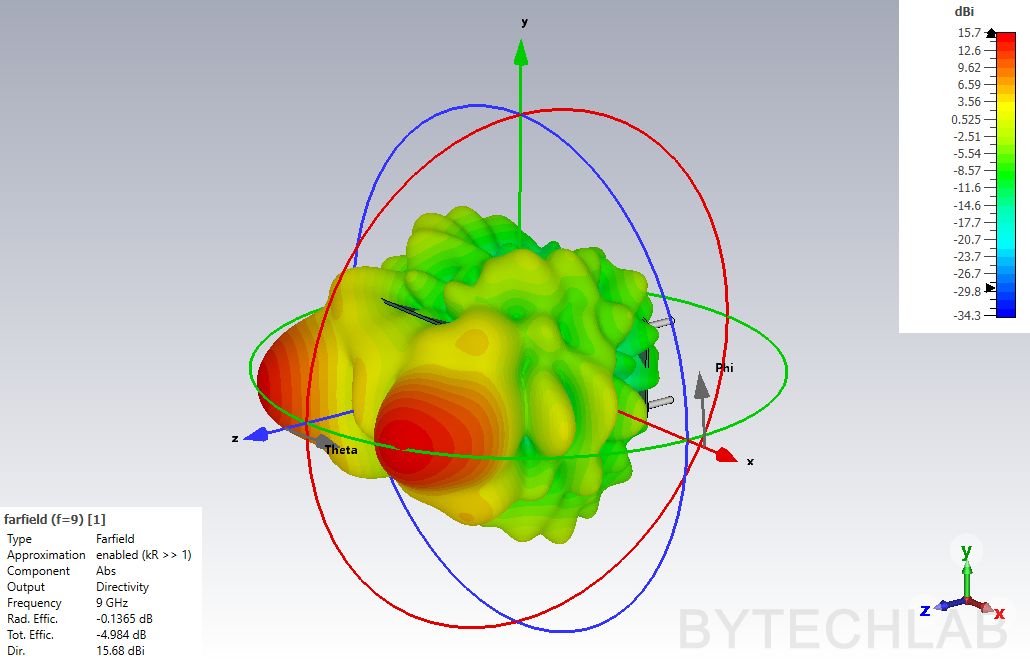
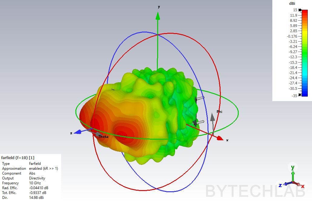
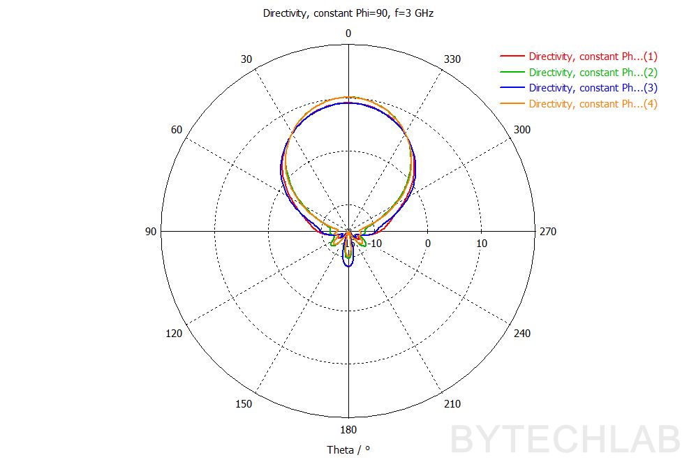
Below you can see also other antenna characteristics such as: Directivity – 2D farfield cuts (phi=0,phi=90), $|S_{11}|$ , Port impedance, Directivity Max., Angular width (phi=0), Side lobe level (Phi =0), Total Efficiency, Realized Gain (phi =0, theta=0).

PCB Coaxial-Fed Horn Antenna (3-7 GHz) - Final simulation – Directivity (Const phi = 90 deg) — Final simulation – Directivity (Const phi = 90 deg)

PCB Coaxial-Fed Horn Antenna (3-7 GHz) - Final simulation – Directivity (Const phi = 0 deg) — Final simulation – Directivity (Const phi = 0 deg)

PCB Coaxial-Fed Horn Antenna (3-7 GHz) - Final simulation – S11 — Final simulation – S11

PCB Coaxial-Fed Horn Antenna (3-7 GHz) - Final simulation – Port impedance — Final simulation – Port impedance

PCB Coaxial-Fed Horn Antenna (3-7 GHz) - Final simulation – Directivity Max. — Final simulation – Directivity Max.

PCB Coaxial-Fed Horn Antenna (3-7 GHz) - Final simulation – Directivity Max (Const phi = 0 deg) — Final simulation – Directivity Max (Const phi = 0 deg)

PCB Coaxial-Fed Horn Antenna (3-7 GHz) - Final simulation - Angular width (Const phi = 0 deg) — Final simulation – Angular width (Const phi = 0 deg)

PCB Coaxial-Fed Horn Antenna (3-7 GHz) - Final simulation – Side lobe level (Const phi = 0 deg) — Final simulation – Side lobe level (Const phi = 0 deg)

PCB Coaxial-Fed Horn Antenna (3-7 GHz) - Final simulation – Total Efficiency — Final simulation – Total Efficiency

PCB Coaxial-Fed Horn Antenna (3-7 GHz) - Final simulation – Realized Gain (Phi =0, Theta=0) — Final simulation – Realized Gain (Phi =0, Theta=0)

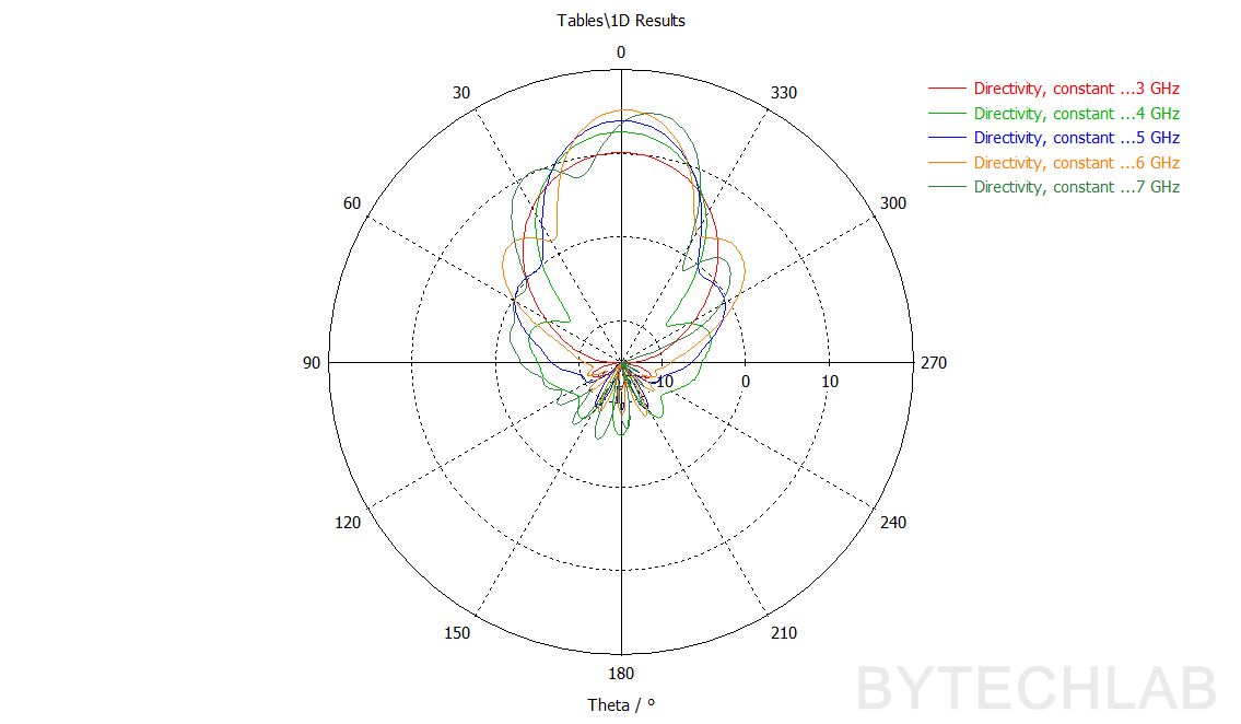
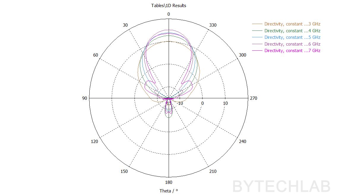
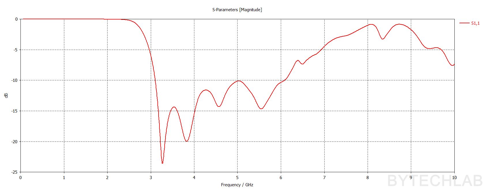
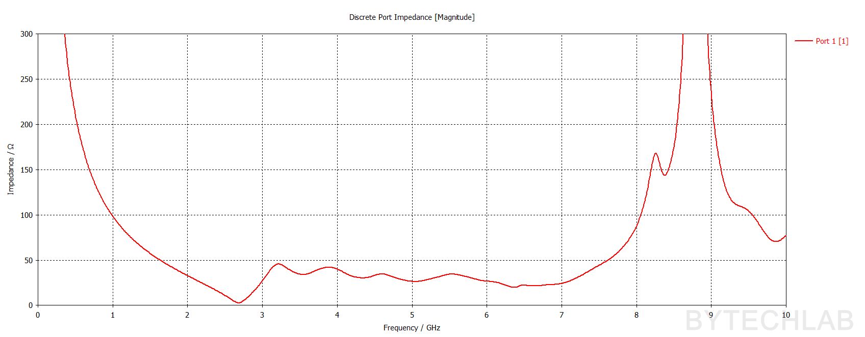
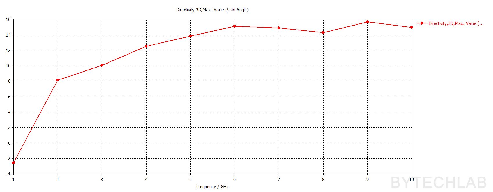
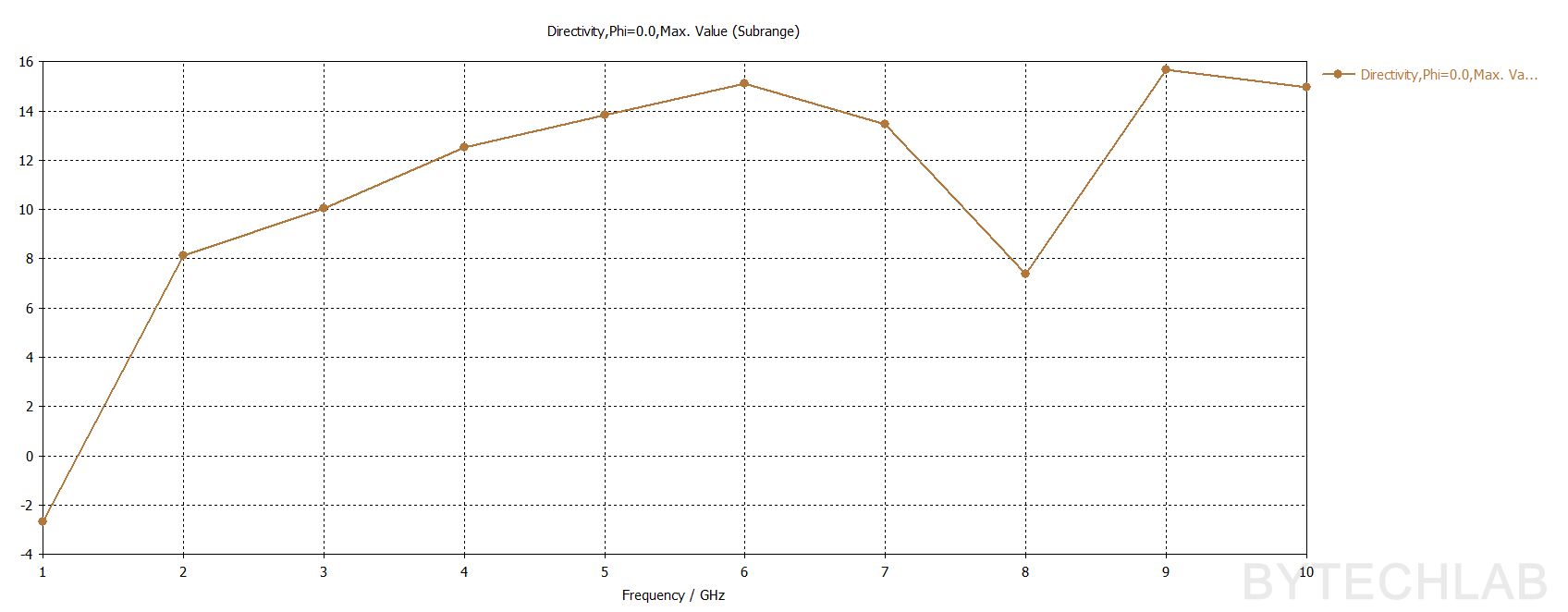
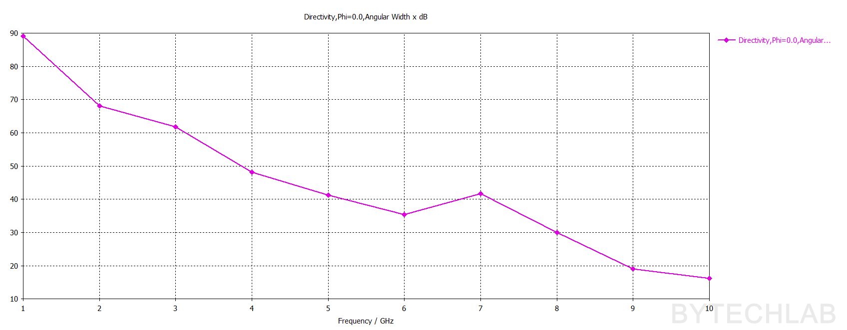
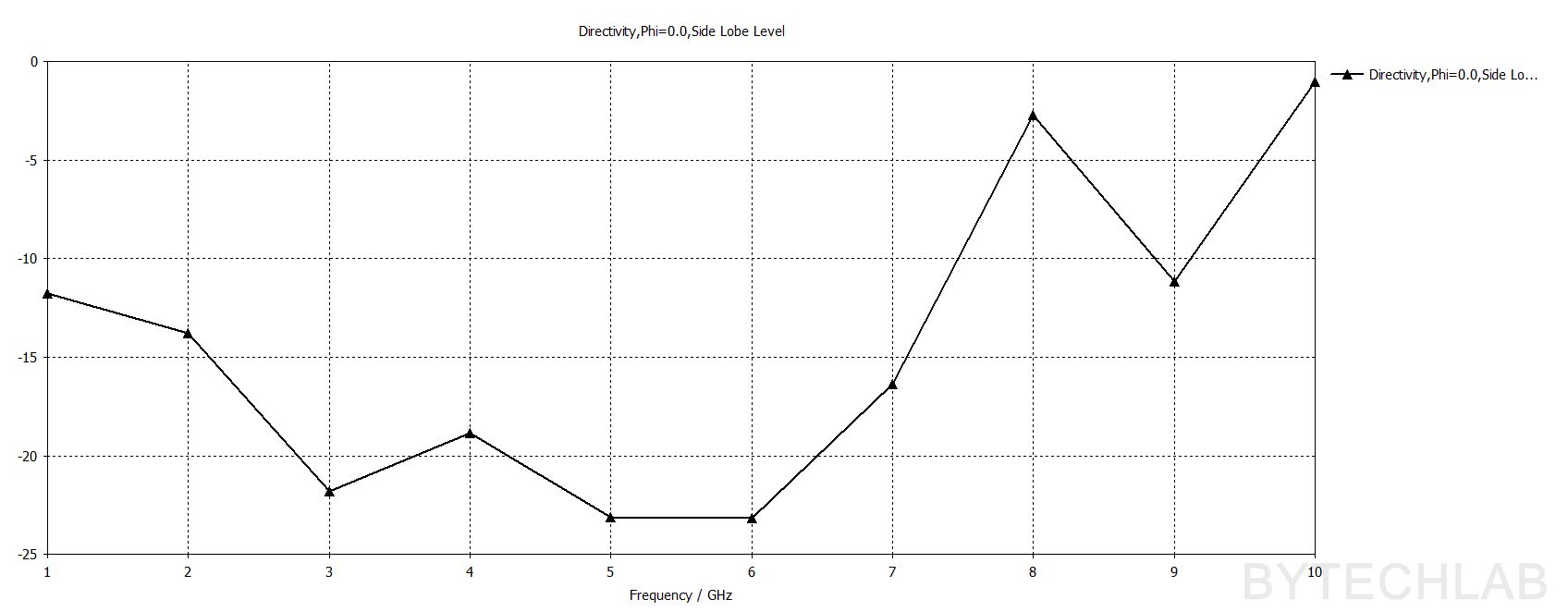
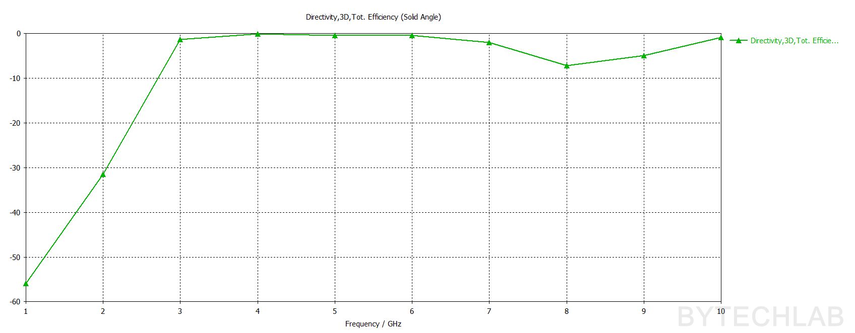
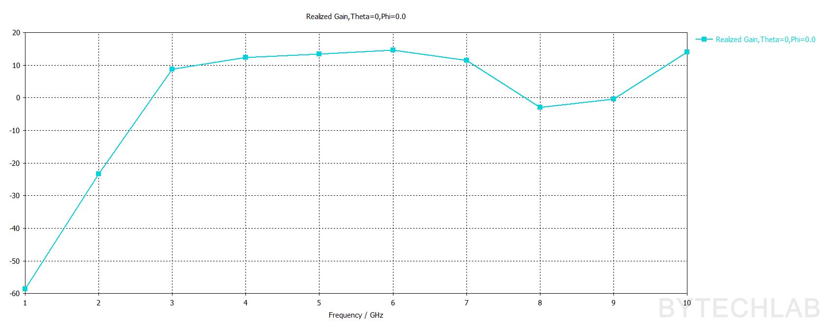
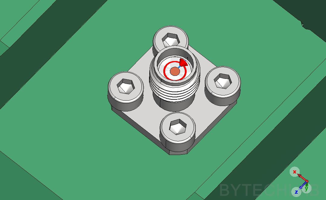
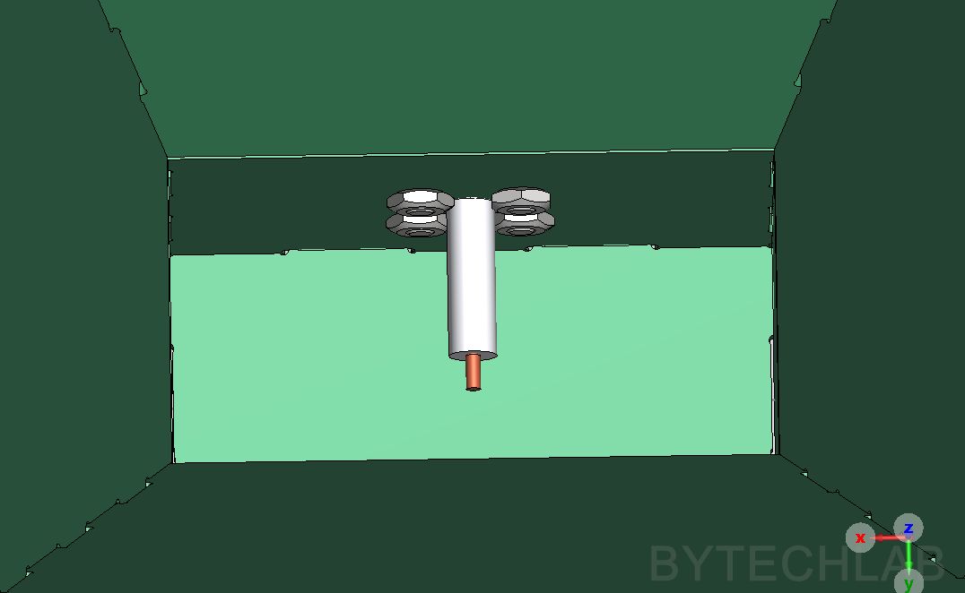
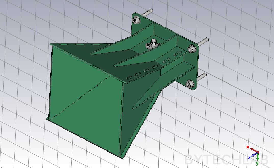
Also on the screens below you can see the port placement and the open boundary box around the antenna:

PCB Coaxial-Fed Horn Antenna (3-7 GHz) - Final simulation – Boundary box — Final simulation – Boundary box

PCB Coaxial-Fed Horn Antenna (3-7 GHz) - Final simulation – Port placement — Final simulation – Port placement

PCB Coaxial-Fed Horn Antenna (3-7 GHz) - Final simulation – 3D model 2 — Final simulation – 3D model 2

PCB Coaxial-Fed Horn Antenna (3-7 GHz) - Final simulation – 3D model — Final simulation – 3D model

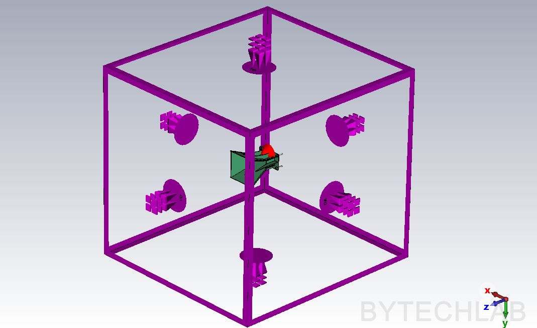
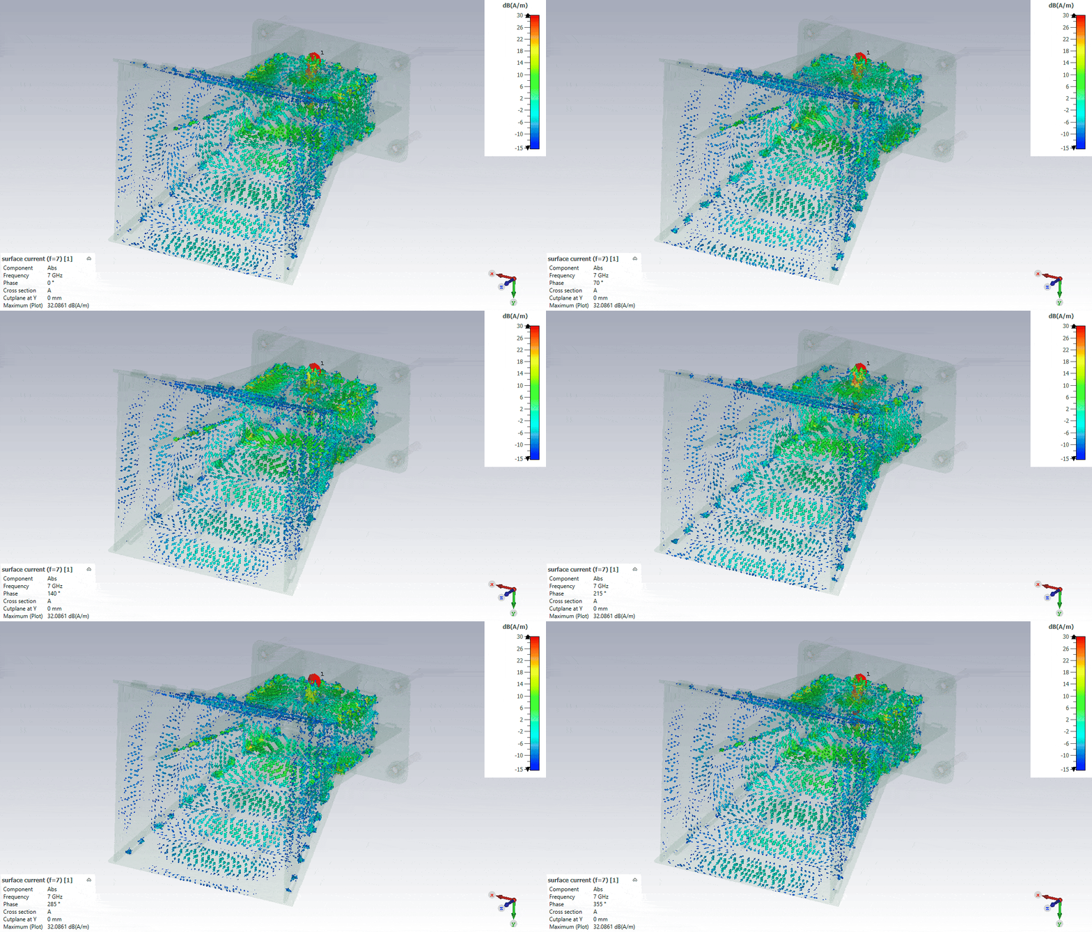
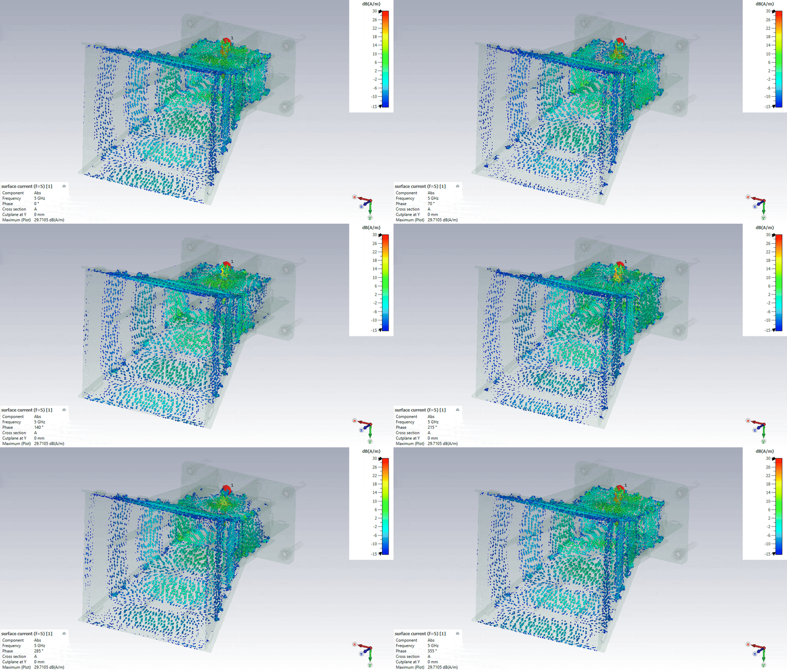
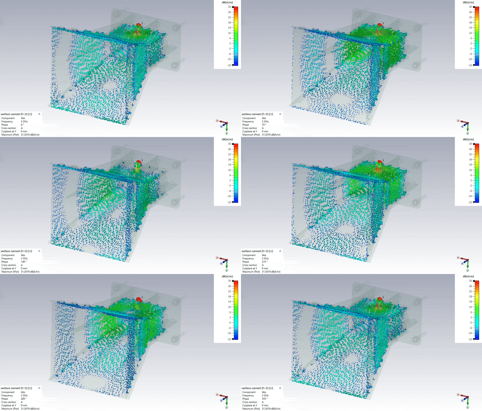
The surface currents are strongest around the probe and in the waveguide section – exactly where the seams have to be soldered most carefully.

PCB Coaxial-Fed Horn Antenna (3-7 GHz) - Final simulation - Surface current - 7 GHz — Final simulation – Surface current – 7 GHz

PCB Coaxial-Fed Horn Antenna (3-7 GHz) - Final simulation - Surface current - 5 GHz — Final simulation – Surface current – 5 GHz

PCB Coaxial-Fed Horn Antenna (3-7 GHz) - Final simulation - Surface current - 3 GHz — Final simulation – Surface current – 3 GHz

Does it work above 7 GHz?

I performed additional simulations up to 10 GHz to check this. This antenna wasn’t designed for these frequencies, so I don’t expect much from it. |S₁₁| is about −4 dB at 7 GHz and gets even worse above, and the beam splits into large side lobes at 8 GHz – exactly what the higher-order modes predict. So above ~7 GHz the antenna is not really usable.

4) Assembly

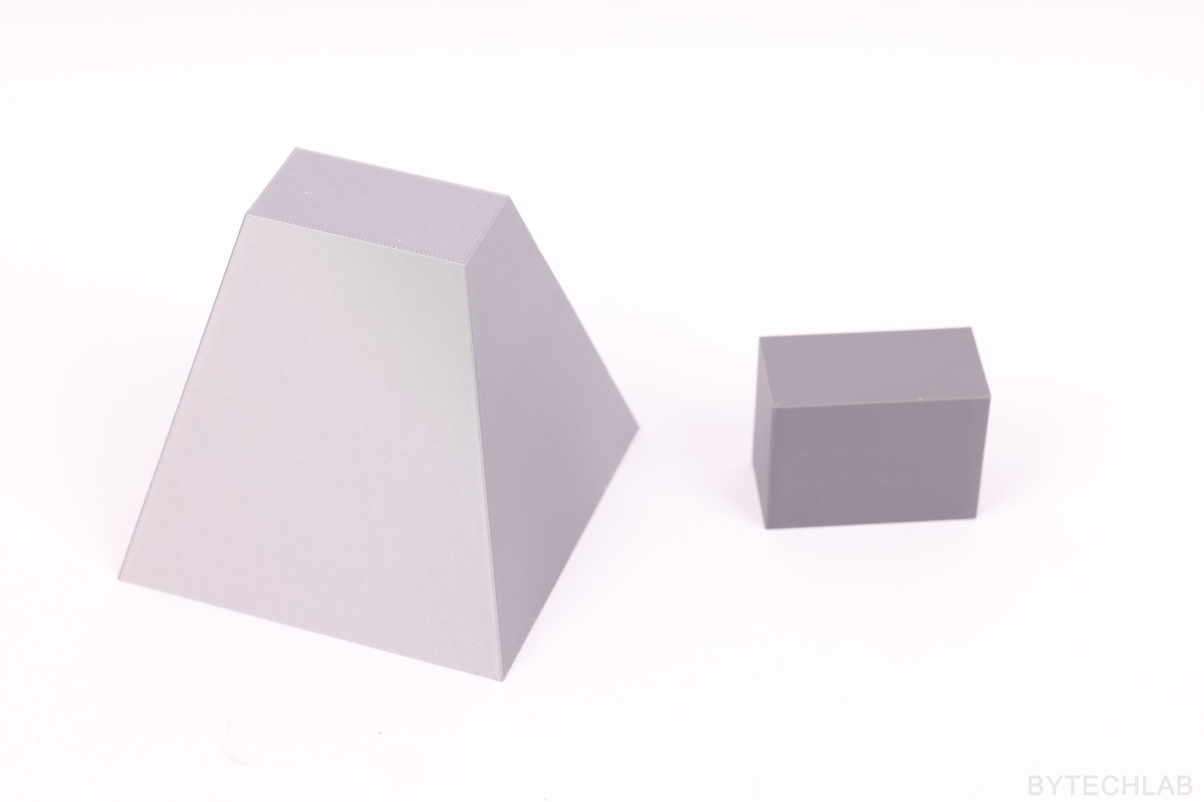
PCB Coaxial-Fed Horn Antenna (3-7 GHz) - Assembly Jig — Assembly Jig

To get the right flare angles, I designed a simple 3D-printed assembly jig with the inner shape of the horn. The PCBs are placed on the jig and soldered while it holds them in position, so every antenna comes out practically identical – important when you want to use several of them in an array. Of course you can find the .STL files in the Github repository.

PCB Coaxial-Fed Horn Antenna (3-7 GHz) - Assembly Jig - 2 — Assembly Jig – 2

PCB Coaxial-Fed Horn Antenna (3-7 GHz) - Assembly Jig - 3 — Assembly Jig – 3

5) Photos

PCB Coaxial-Fed Horn Antenna (3-7 GHz) - Assembled - Multiple antennas — Assembled – Multiple antennas

PCB Coaxial-Fed Horn Antenna (3-7 GHz) - Assembled - SMA connector — Assembled – SMA connector

PCB Coaxial-Fed Horn Antenna (3-7 GHz) - Assembled - Side view 2 — Assembled – Side view 2

PCB Coaxial-Fed Horn Antenna (3-7 GHz) - Assembled - Side view — Assembled – Side view

PCB Coaxial-Fed Horn Antenna (3-7 GHz) - Assembled - Rear view 2 — Assembled – Rear view 2

PCB Coaxial-Fed Horn Antenna (3-7 GHz) - Assembled - Rear view — Assembled – Rear view

PCB Coaxial-Fed Horn Antenna (3-7 GHz) - Assembled - Front view — Assembled – Front view

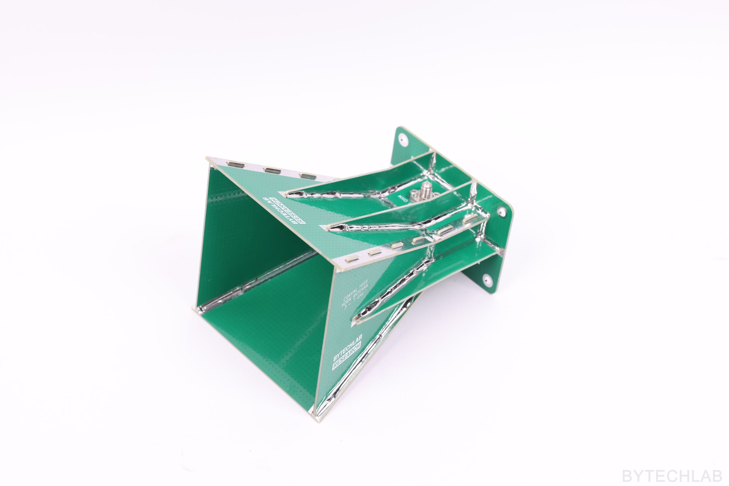
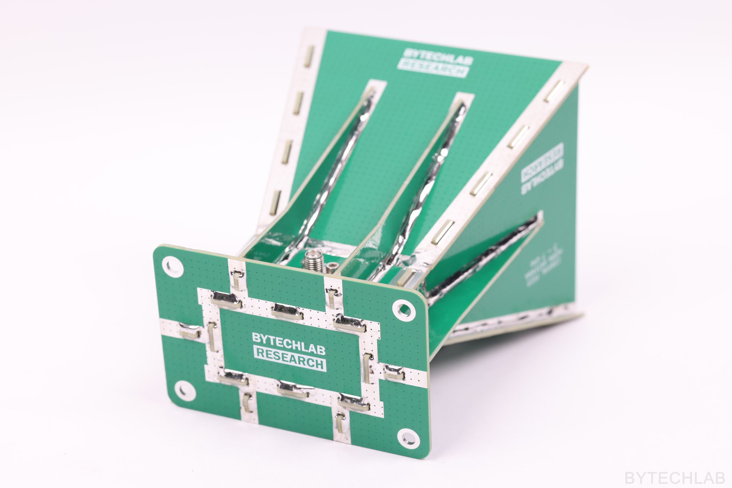
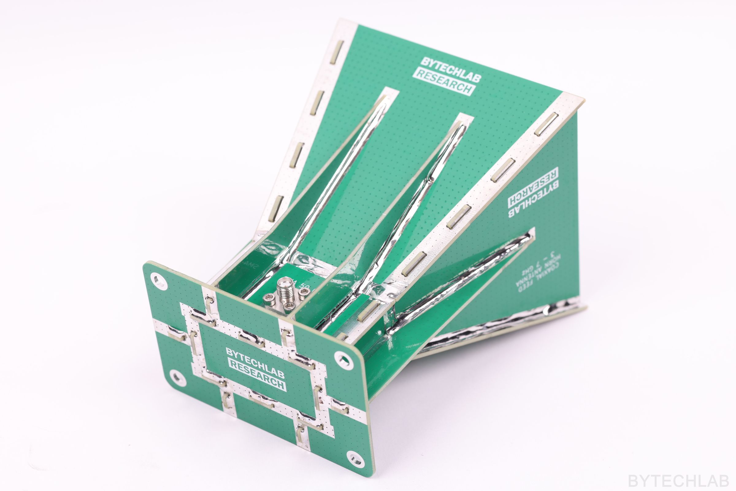
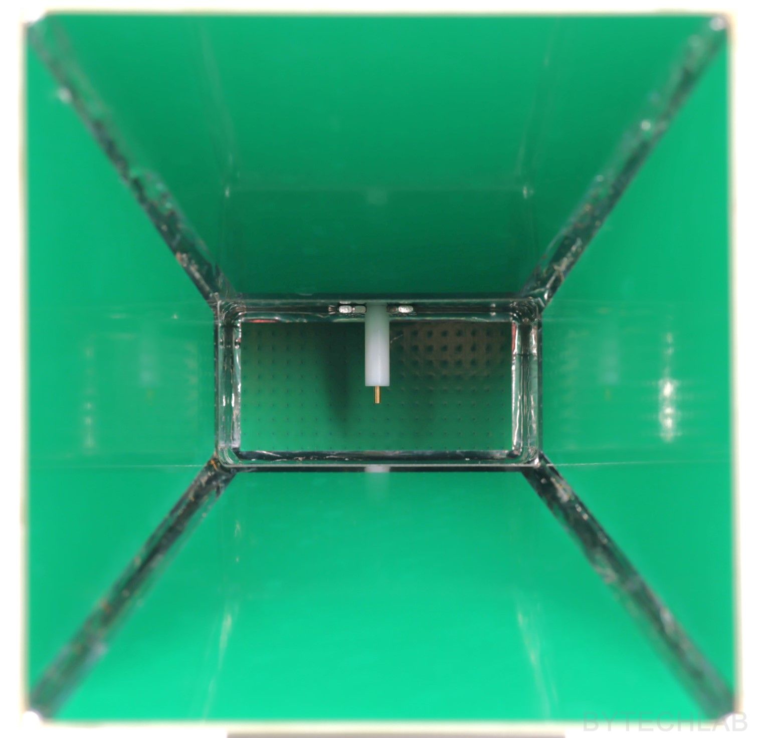
6) Measurements

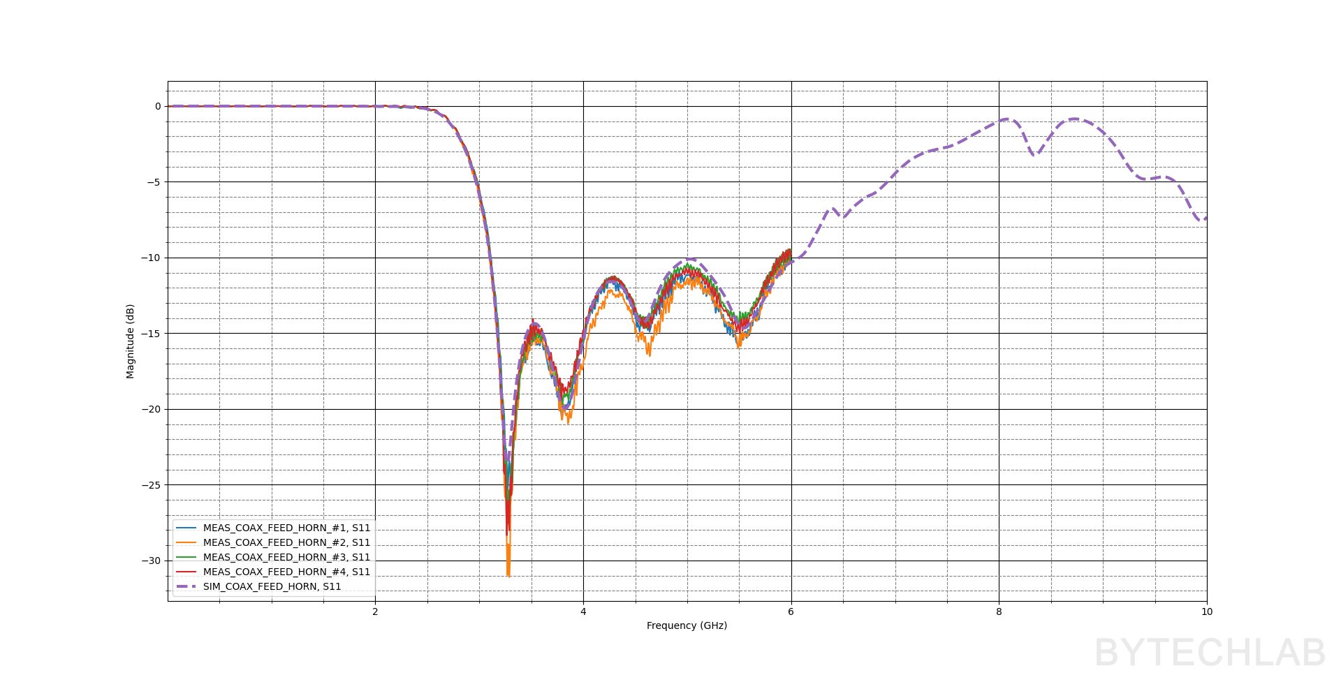
PCB Coaxial-Fed Horn Antenna (3-7 GHz) - Simulation vs. Measurement - S11 (LogMag) — Simulation vs. Measurement – S11 (LogMag)

I have measured the S-parameters with my LibreVNA. The measured |S₁₁| of all four antennas matches the simulation very well, and the antennas are almost identical (only #2 differs slightly). |S₁₁| is below −10 dB across most of the measured range and better than -5 dB in the whole operating range (3-7 GHz). My VNA only goes up to 6 GHz, so the 6–7 GHz part is covered by the simulation (dashed line): the matching gets gradually worse there, to about −7 dB at 6.5 GHz. So the antenna works best between 3 and 6 GHz, and it still works – just not as well – up to 7 GHz. The small differences most likely come from the small differences in mechanical dimensions due to manual assembly process.

I measured the radiation patterns outdoors with my antenna positioner at 3, 4, 5 and 6 GHz. Basically it a mechanical device (made from dielectric materials) that rotates the antenna in 3D (two axes). To measure the radiation patterns I’m using a second wideband reference antenna placed on a stand. Both antennas are hooked up to a two-port VNA and a laptop with a script that controls everything. I will publish post about that soon!

For a proper far-field measurement the antennas have to be further apart than [1]:

\begin{array}{c} R_{ff} = \frac{2D^{2}}{\lambda_0} \approx 0.75\ \mathrm{m}\ \ (D = 136.7\ \mathrm{mm},\ 6\ \mathrm{GHz}) \qquad (5) \\ \scriptstyle \text{Source: [1] Sec. 2.2.4} \end{array}

where D is the largest aperture dimension (the diagonal). In my setup the distance was about 1m (I had to put the antennas close together because of poor dynamic range of libreVNA at higher frequencies). Each measured pattern is normalized to the simulated peak value shown in the plot title.

PCB Coaxial-Fed Horn Antenna (3-7 GHz) - Simulation vs. Measurement - Radiation Pattern (Azimuth cut, 3 GHz) — Simulation vs. Measurement – Radiation Pattern (Azimuth cut, 3 GHz)

PCB Coaxial-Fed Horn Antenna (3-7 GHz) - Simulation vs. Measurement - Radiation Pattern (Elevation cut, 3 GHz) — Simulation vs. Measurement – Radiation Pattern (Elevation cut, 3 GHz)

PCB Coaxial-Fed Horn Antenna (3-7 GHz) - Simulation vs. Measurement - Radiation Pattern (Azimuth cut, 4 GHz) — Simulation vs. Measurement – Radiation Pattern (Azimuth cut, 4 GHz)

PCB Coaxial-Fed Horn Antenna (3-7 GHz) - Simulation vs. Measurement - Radiation Pattern (Elevation cut, 4 GHz) — Simulation vs. Measurement – Radiation Pattern (Elevation cut, 4 GHz)

PCB Coaxial-Fed Horn Antenna (3-7 GHz) - Simulation vs. Measurement - Radiation Pattern (Azimuth cut, 5 GHz) — Simulation vs. Measurement – Radiation Pattern (Azimuth cut, 5 GHz)

PCB Coaxial-Fed Horn Antenna (3-7 GHz) - Simulation vs. Measurement - Radiation Pattern (Elevation cut, 5 GHz) — Simulation vs. Measurement – Radiation Pattern (Elevation cut, 5 GHz)

PCB Coaxial-Fed Horn Antenna (3-7 GHz) - Simulation vs. Measurement - Radiation Pattern (Azimuth cut, 6 GHz) — Simulation vs. Measurement – Radiation Pattern (Azimuth cut, 6 GHz)

PCB Coaxial-Fed Horn Antenna (3-7 GHz) - Simulation vs. Measurement - Radiation Pattern (Elevation cut, 6 GHz) — Simulation vs. Measurement – Radiation Pattern (Elevation cut, 6 GHz)

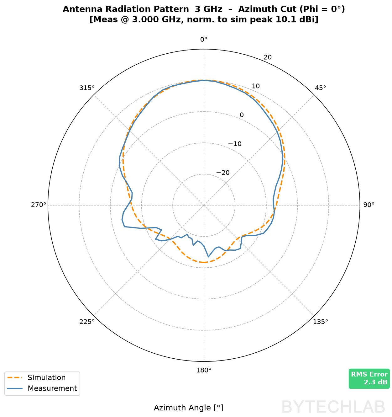
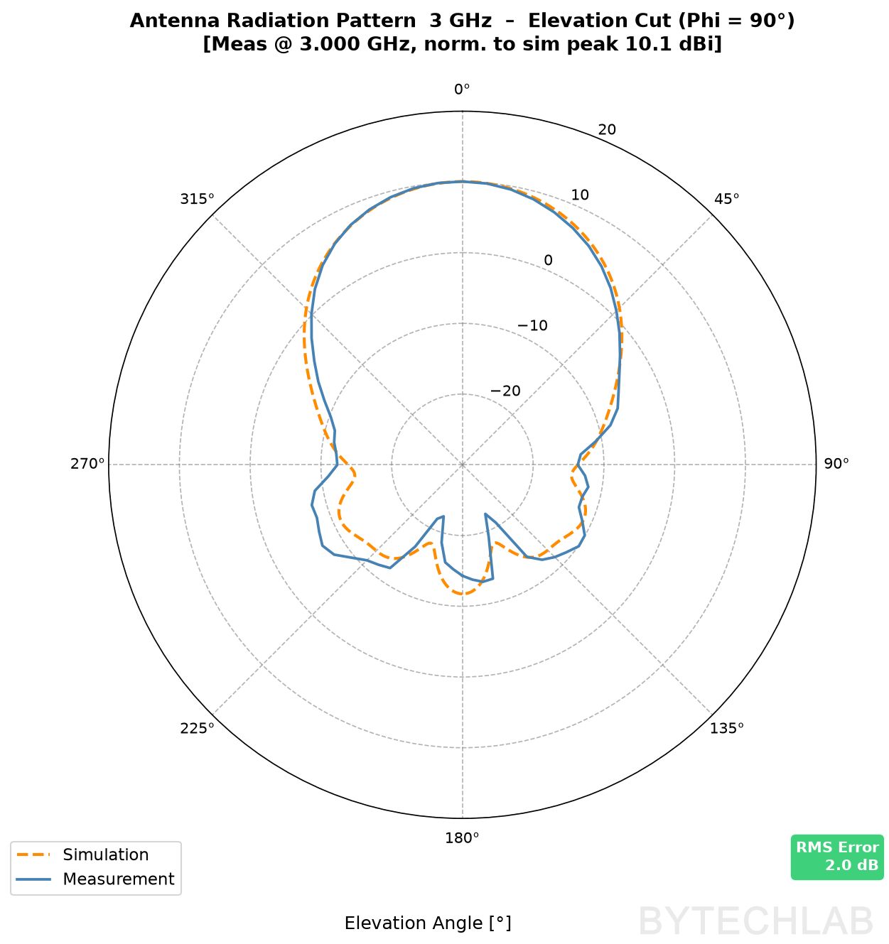
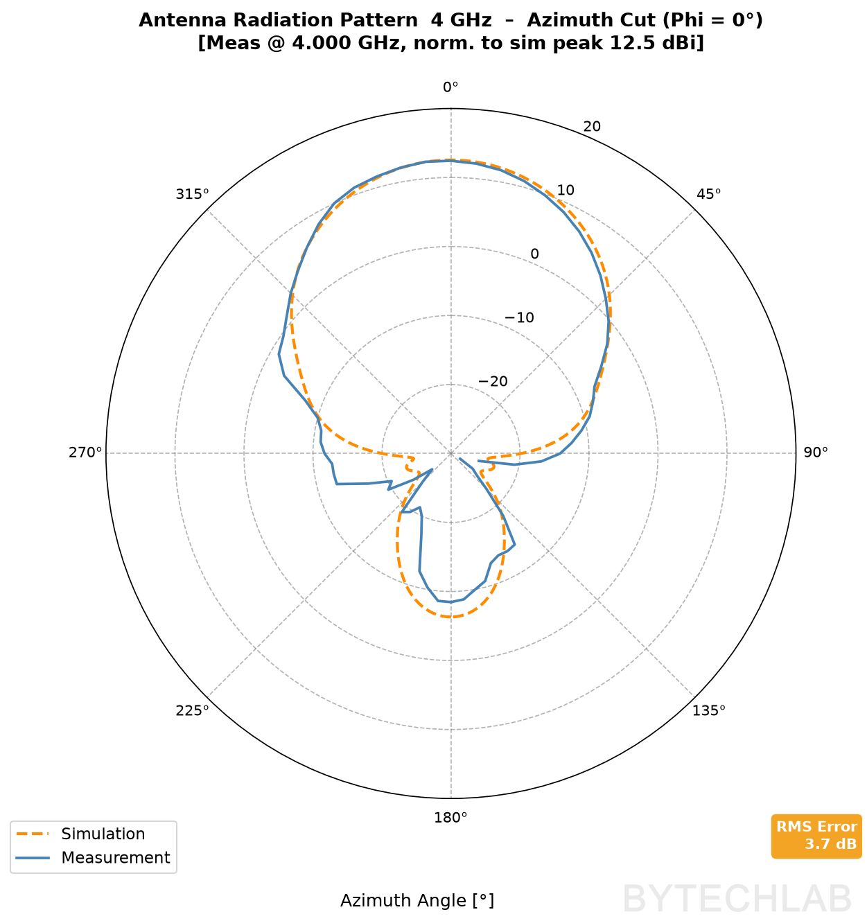
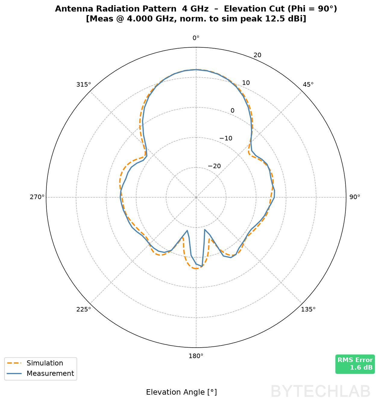
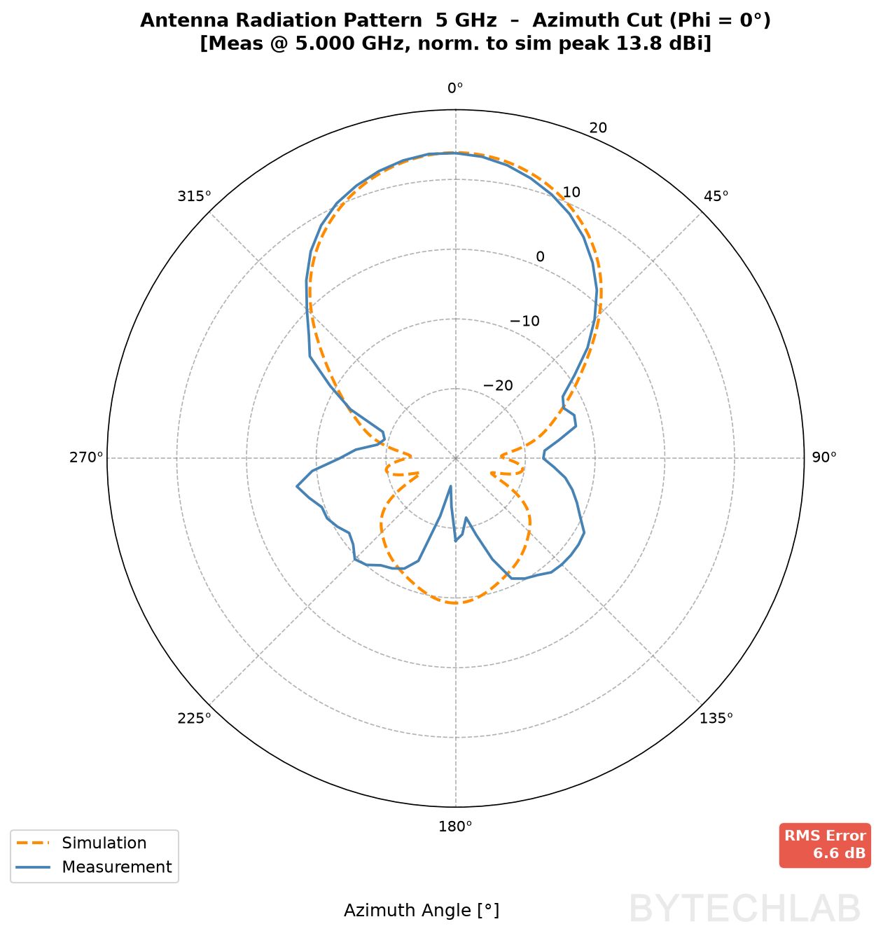
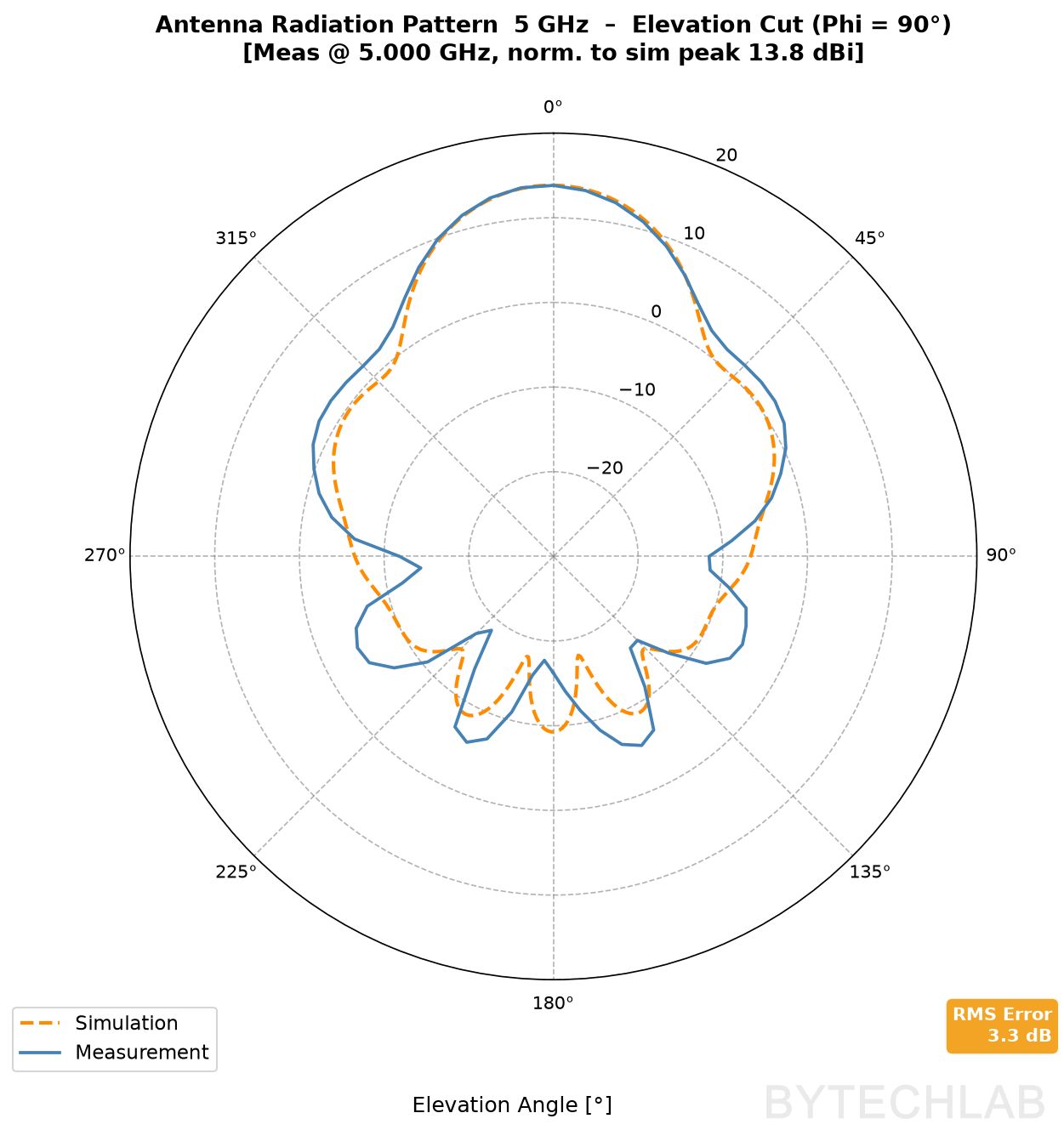
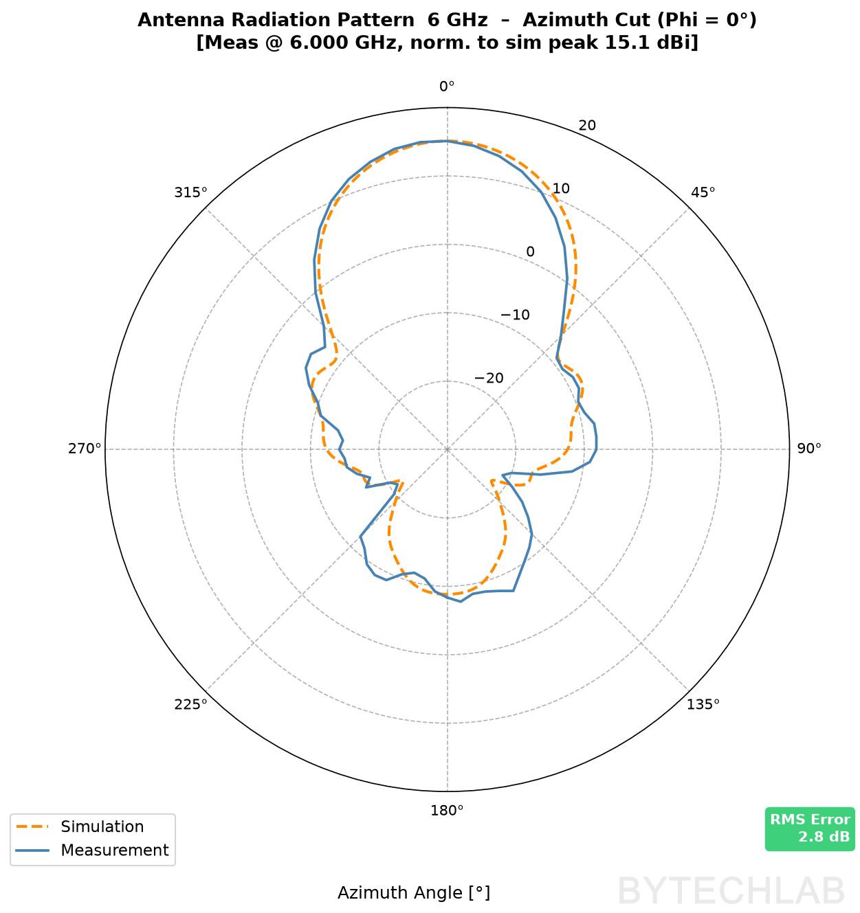
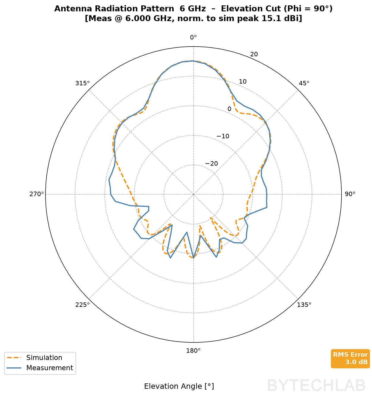
The main lobe matches the simulation very well at all frequencies in both planes. The RMS error (1.6–6.6 dB) comes almost entirely from the side and back lobes, 20–30 dB below the peak, which are easily affected by reflections from the ground, trees, the mast and the positioner during an outdoor measurement. The worst case is the 5 GHz azimuth cut, but the elevation cut at the same frequency looks much better, so I’d blame the environment rather than the antenna ( I don’t have an anechoic chamber yet). For the radar, the main lobe is what matters, and it’s reproduced well. Overall I’m amazed how well that works given that the measurement setup is far from ideal.

On the video below you can see how the antenna positioner rotates the antenna around it’s center of rotation.

Below you can see the full measured 3D pattern – use the slider to change the frequency. This the real measured interactive 3D radiation pattern that you can rotate with your mouse!

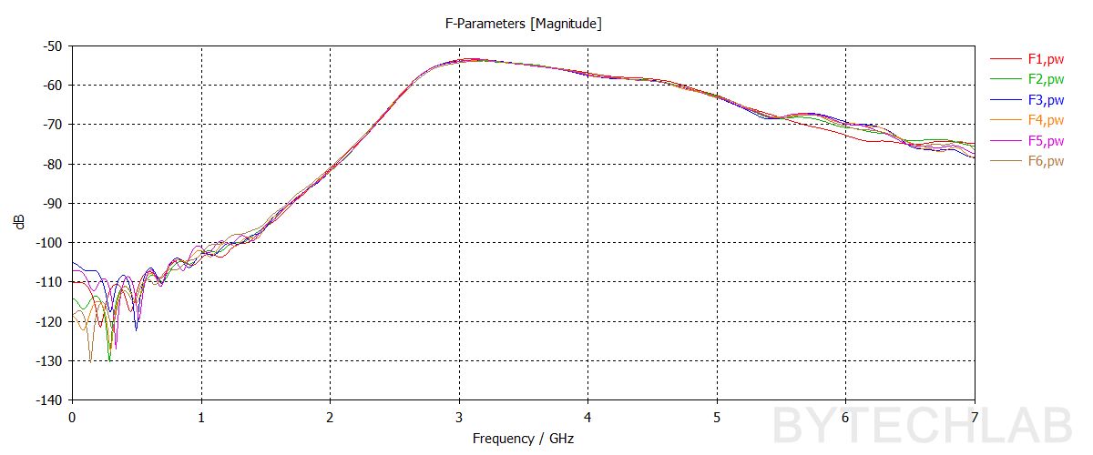
7) 1D Phased array simualtions – 0 deg. wavefront

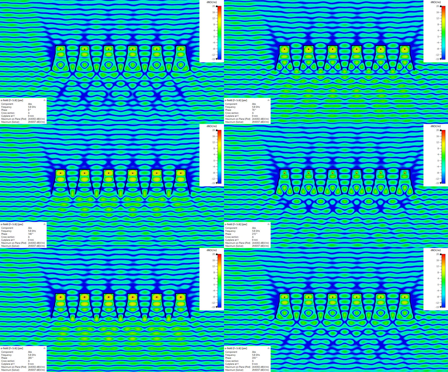
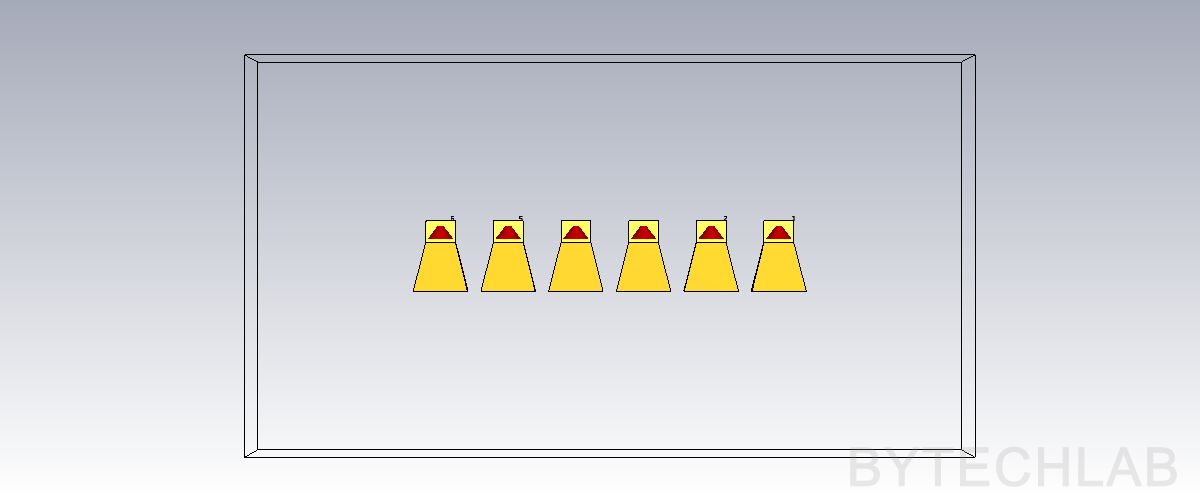
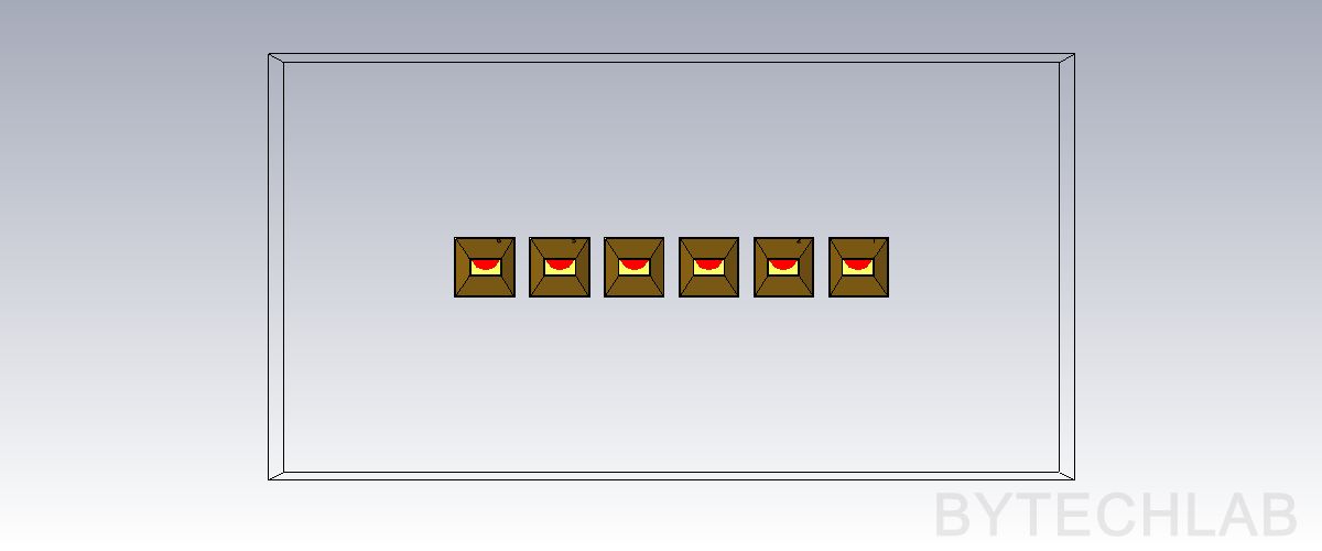
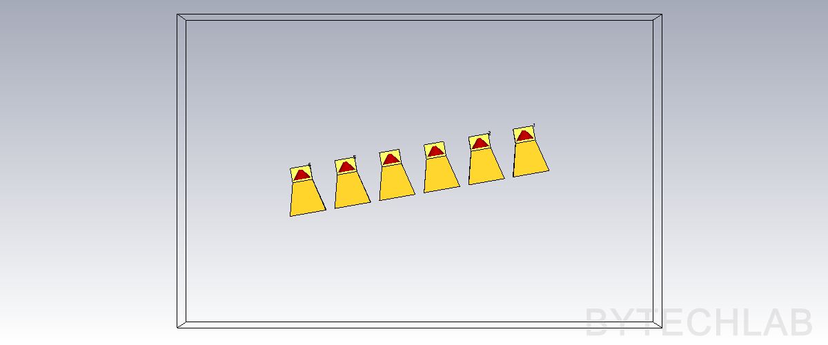
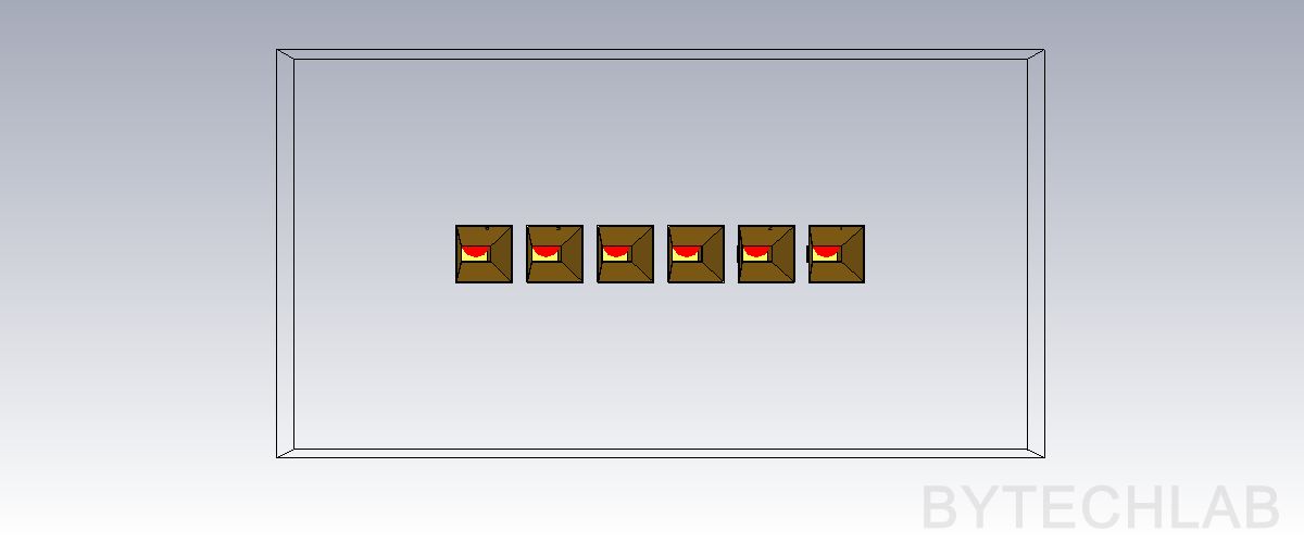
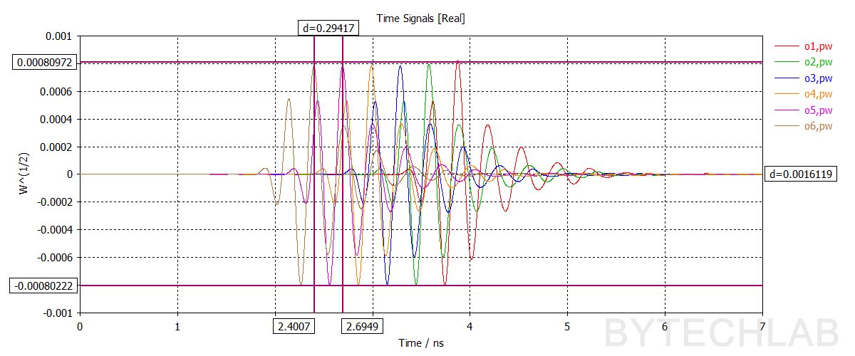
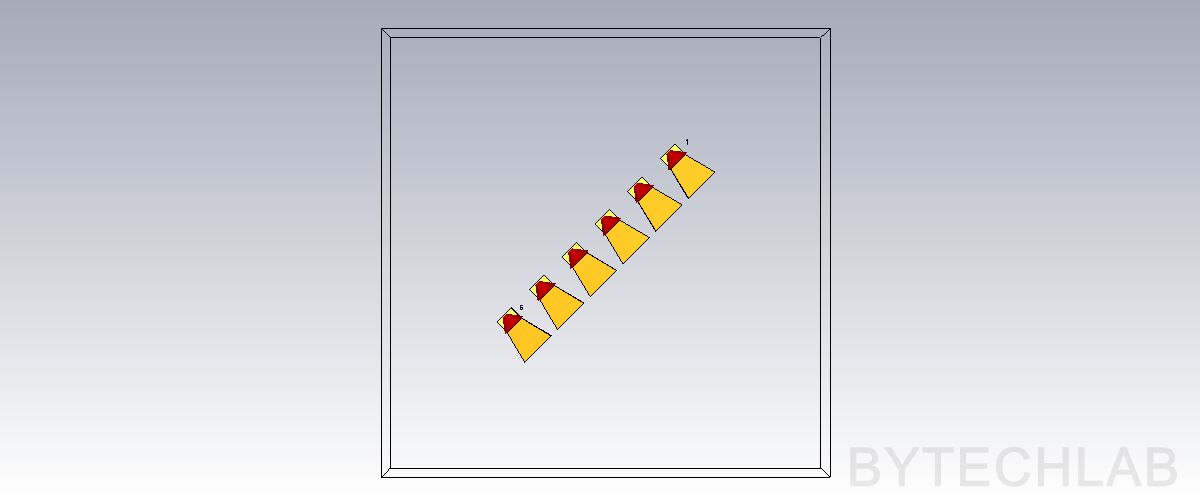
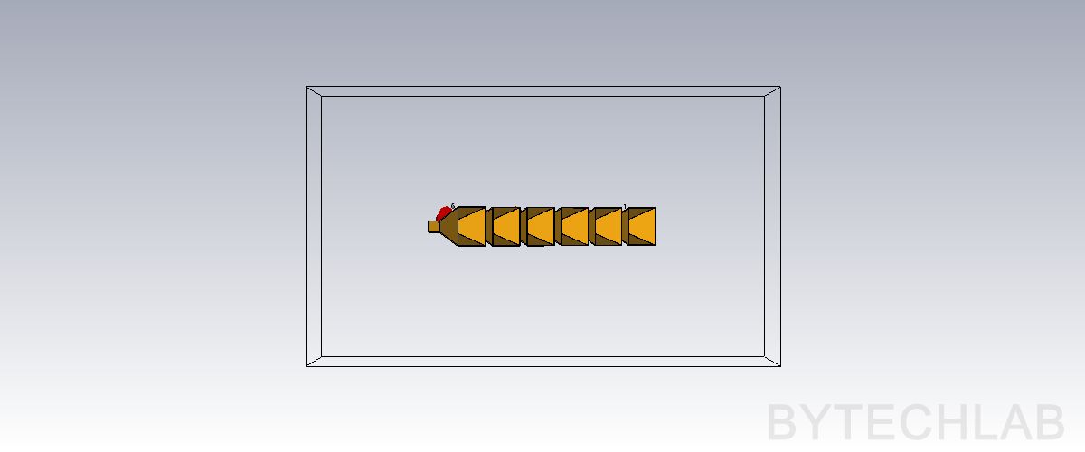
PCB Coaxial-Fed Horn Antenna (3-7 GHz) - Phased array simulation - 0 deg. - E field animation — Phased array simulation – 0 deg. – E field animation

In my radar one antenna will transmit and the others will work as separate receivers. The direction of a reflection is calculated from the differences in time of arrival of the returning wave at each receiver. To check this, I simulated six horns spaced d = 125 mm apart, illuminated by a plane wave at 5.8 GHz. A wave arriving at angle θ reaches neighbouring receivers with a delay of:

\begin{array}{c} \Delta t = \frac{d\,\sin\theta}{c} \qquad (6) \\ \scriptstyle \text{Source: [1] eq. (6-7a)} \end{array}

Balanis [1] writes the phase difference between neighbouring array elements with the angle measured from the array axis and with an extra feed phase β. For my receivers the angle is measured from boresight and there is no extra phase, so the phase difference turns into a time delay by dividing by 2πf.

\begin{array}{c} \begin{aligned} \psi &= k d \cos\theta’ + \beta && \text{[1] eq. (6-7a), } \theta’ \text{ measured from the array axis} \\ \cos\theta’ &= \sin\theta && \theta = 90^{\circ} – \theta’ \text{ measured from boresight} \\ \Delta\varphi &= k d \sin\theta = 2\pi\,\frac{d\sin\theta}{\lambda_0} && \text{receive only: } \beta = 0 \\ \Rightarrow\ \Delta t &= \frac{\Delta\varphi}{2\pi f} = \frac{d\sin\theta}{\lambda_0 f} = \frac{d\sin\theta}{c} && \end{aligned} \\ \scriptstyle \text{Derivation of eq. (6)} \end{array}

PCB Coaxial-Fed Horn Antenna (3-7 GHz) - Phased array simulation - 0 deg. - F parameters — Phased array simulation – 0 deg. – F parameters

PCB Coaxial-Fed Horn Antenna (3-7 GHz) - Phased array simulation - 0 deg. - Port signals — Phased array simulation – 0 deg. – Port signals

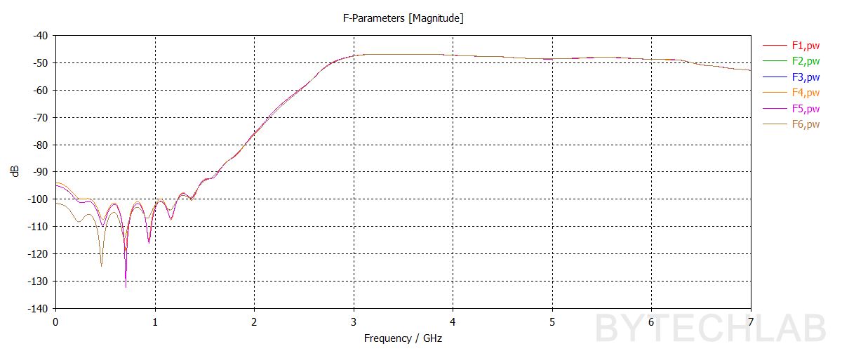
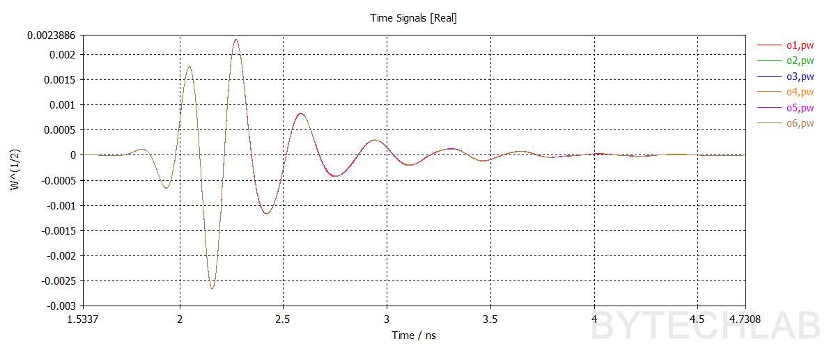
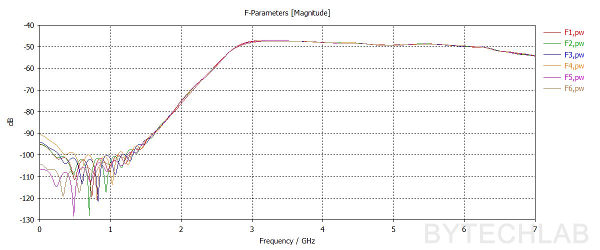
At 0° all receivers see the wave at the same time – the port signals overlap perfectly. To do these simulation’s I’m using a Time Domain solver (TD) with a broadband pulse excitation.

PCB Coaxial-Fed Horn Antenna (3-7 GHz) - Phased array simulation - 0 deg. - 3D Model — Phased array simulation – 0 deg. – 3D Model

PCB Coaxial-Fed Horn Antenna (3-7 GHz) - Phased array simulation - 0 deg. - 3D Model 2 — Phased array simulation – 0 deg. – 3D Model 2

8) 1D Phased array simualtions – 10 deg. wavefront

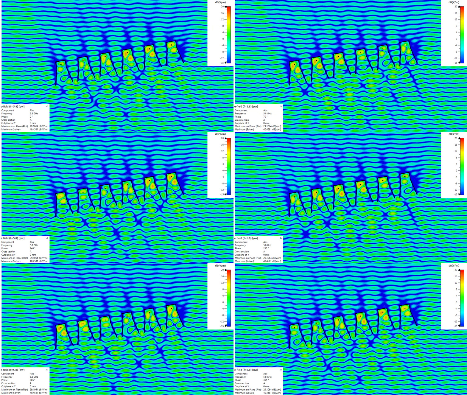
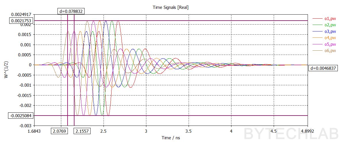
PCB Coaxial-Fed Horn Antenna (3-7 GHz) - Phased array simulation - 10 deg. - E field animation — Phased array simulation – 10 deg. – E field animation

At 10° equation (6) gives 72 ps between neighbouring receivers. The markers in the port signal plot show 78.8 ps, which is close enough. Take a look at all of the amazing electromagnetic effect that happen in the antennas and near them !

PCB Coaxial-Fed Horn Antenna (3-7 GHz) - Phased array simulation - 10 deg. - F parameters — Phased array simulation – 10 deg. – F parameters

PCB Coaxial-Fed Horn Antenna (3-7 GHz) - Phased array simulation - 10 deg. - Port signals — Phased array simulation – 10 deg. – Port signals

PCB Coaxial-Fed Horn Antenna (3-7 GHz) - Phased array simulation - 10 deg. - 3D Model — Phased array simulation – 10 deg. – 3D Model

PCB Coaxial-Fed Horn Antenna (3-7 GHz) - Phased array simulation - 10 deg. - 3D Model 2 — Phased array simulation – 10 deg. – 3D Model 2

9) 1D Phased array simualtions – 30 deg. wavefront

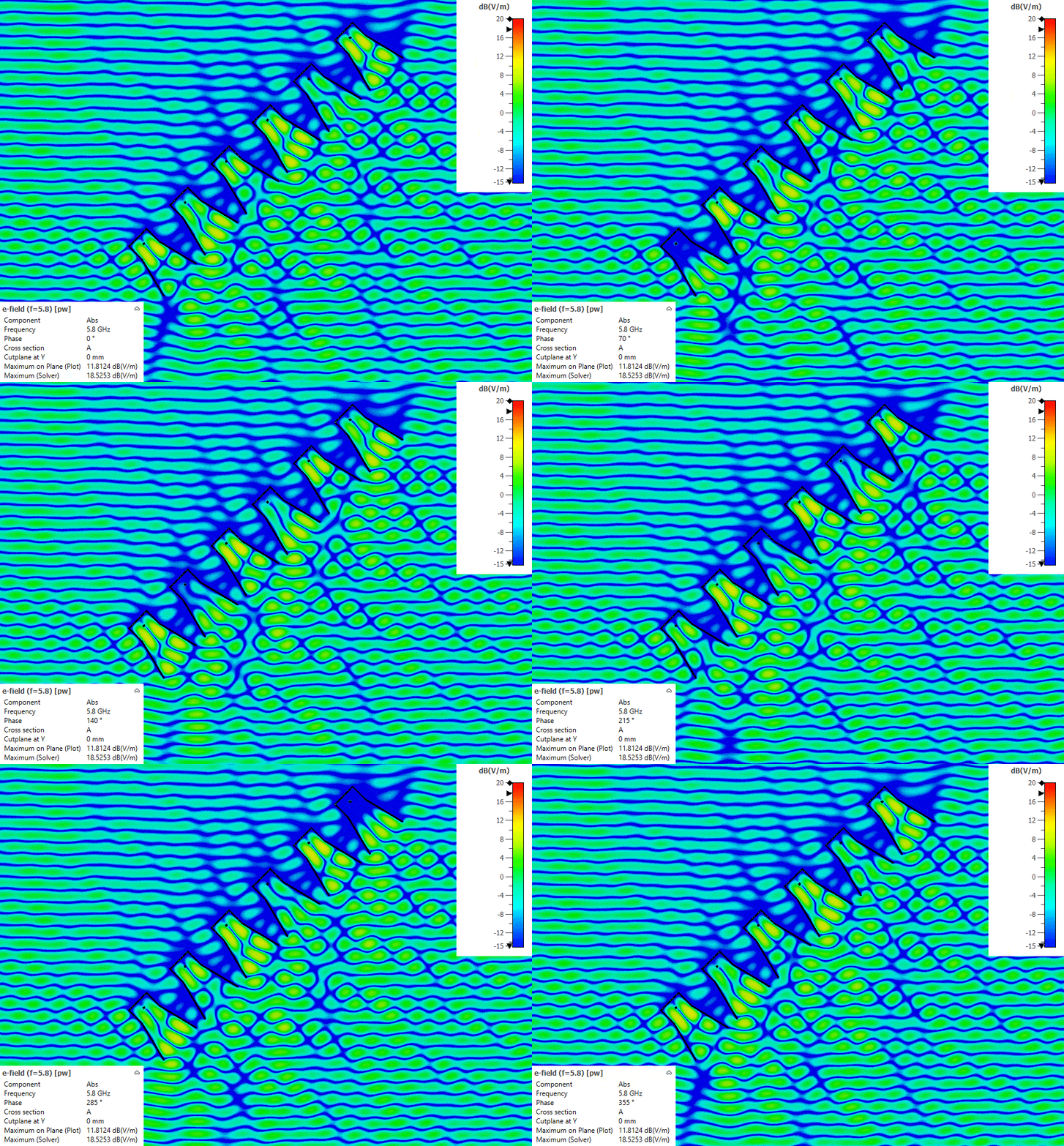
PCB Coaxial-Fed Horn Antenna (3-7 GHz) - Phased array simulation - 30 deg. - E field animation — Phased array simulation – 30 deg. – E field animation

At 30° the delay grows to ~280ps. This is a good moment to mention one important limitation. At 5.8 GHz one period of the wave lasts only 172 ps, so the 280 ps delay is more than a full period. If you only compared the phase of the signals, you’d see just the leftover 108 ps and get a completely wrong angle. With my 125 mm spacing, phase alone is unambiguous only within ±12° [1]. Because the horns are big, I can’t put them closer together. The solution is to measure the real delay of the signal envelope, not just the phase.

PCB Coaxial-Fed Horn Antenna (3-7 GHz) - Phased array simulation - 30 deg. - F parameters — Phased array simulation – 30 deg. – F parameters

PCB Coaxial-Fed Horn Antenna (3-7 GHz) - Phased array simulation - 30 deg. - Port signals — Phased array simulation – 30 deg. – Port signals

PCB Coaxial-Fed Horn Antenna (3-7 GHz) - Phased array simulation - 30 deg. - 3D Model — Phased array simulation – 30 deg. – 3D Model

PCB Coaxial-Fed Horn Antenna (3-7 GHz) - Phased array simulation - 30 deg. - 3D Model 2 — Phased array simulation – 30 deg. – 3D Model 2

8) Antenna Specification

Antenna size [mm]	106.97 × 99.52 × 132.57 (incl. tabs and back plate)
Antenna type	Directional, pyramidal horn, coaxial-probe fed
Frequency range	3–6 GHz with very good performance; still usable up to 7 GHz with worse matching
Antenna gain	10–15 dBi (simulated)
Worst-case efficiency in band	-1 dB in most of the operating band
Polarization	Linear
\|S₁₁\|	< −10 dB across the whole measured range 3–6 GHz (VNA limit)
Cost	~15–20 USD

9) Conclusions

I’m very happy with this antenna. It works really well from 3 to 6 GHz and is still usable up to 7 GHz, where the matching gets worse (|S₁₁| around −4 dB at 7 GHz). It has 10–15 dBi of gain, the measurements agree well with the simulations, and even simple textbook theory predicts its gain within 0.5 dB. Most importantly for my radar project, it’s cheap (~15–20 USD) and fast to build (~1 hour), and thanks to the PCB tolerances and the assembly jig all antennas come out practically identical. Compared to my 3D printed double ridged horn it has a narrower bandwidth, but there’s no painting, no sanding and no long prints. Its limits come directly from the waveguide size: below ~2.9 GHz it doesn’t radiate, and above ~6.3 GHz unwanted modes start to appear.

10) References

[1] C. A. Balanis, Antenna Theory: Analysis and Design, 4th ed., Wiley, 2016.
[2] H. Kumar and G. Kumar, “Coaxial Feed Pyramidal Horn Antenna with High Efficiency,” IETE Journal of Research, vol. 64, no. 1, pp. 51–58, 2018, doi: 10.1080/03772063.2017.1323563.
[3] D. Sablić-Nemec and M. Joler, “An Automated Approach to Horn Antenna Impedance Matching and Manufacturing Using 3D Printing,” Journal of Communications Software and Systems, vol. 19, no. 3, pp. 188–198, 2023, doi: 10.24138/jcomss-2023-0100.
[4] R. P. Jadhav, V. J. Dongre and A. Heddallikar, “Design of X-Band Conical Horn Antenna Using Coaxial Feed and Improved Design Technique for Bandwidth Enhancement,” ICCUBEA 2017, Pune, India, 2017.
[5] A. Alam, S. Urooj and A. Q. Ansari, “Design and Simulation of 24 GHz High Gain Pyramidal Horn Antenna for Bio-Radar Sensing Application,” REEDCON 2023, doi: 10.1109/REEDCON57544.2023.10151440.
[6] D. M. Pozar, Microwave Engineering, 4th ed., Wiley, 2012.
[7] S. Gezici et al., “Localization via ultra-wideband radios: a look at positioning aspects of future sensor networks,” IEEE Signal Processing Magazine, vol. 22, no. 4, pp. 70–84, 2005, doi: 10.1109/MSP.2005.1458289.
[8] Amphenol RF, 901-2PF705590AM SMA panel jack (4-hole flange, 0.705″ post, 0.590″ PTFE), datasheet.

GitHub Repository:

https://github.com/ByTechLab/RF—PCB-Coaxial-Fed-Horn-Antenna–3-7-GHz-