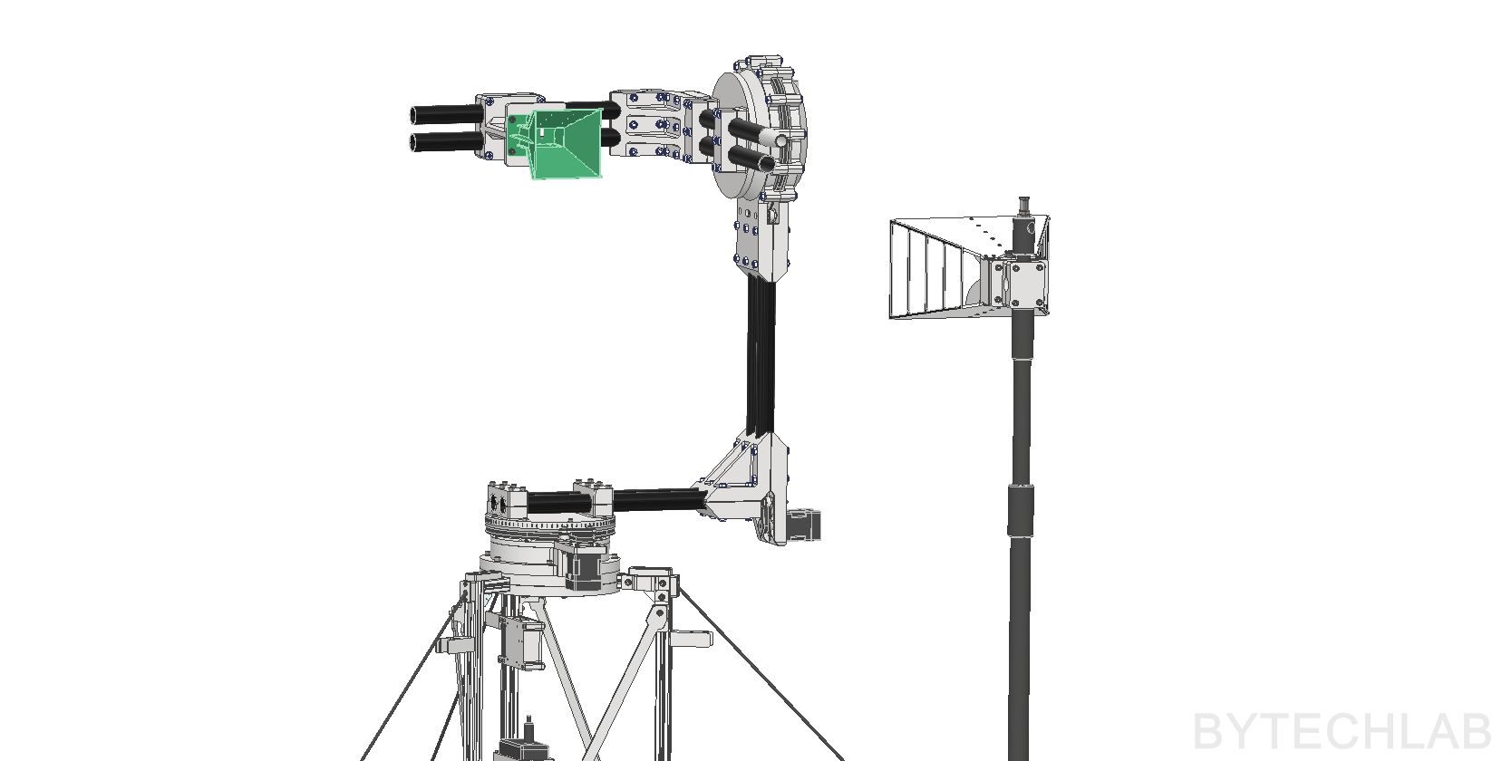
Recently I have designed many antennas, and I thought that it would be nice to be able to measure things other than S11 on site (like radiation patterns). A VNA connected to a single antenna tells you how well it is matched, but nothing about where it radiates. To measure a radiation pattern you need a second antenna, a fixed distance between the two, and a way to point the antenna under test (DUT) in every direction while the VNA records the transmission between them. In a lab this is done in an anechoic chamber with a commercial positioner. I have neither, so I built this Antenna Positioner that I can carry into my garden.
The project is a mix of everything I usually do. The mechanical parts are mostly 3D printed, axes are driven with belts and closed-loop stepper motor. A small PCB connects two MKS SERVO42D closed-loop motors to a CAN bus. A LibreVNA is the measuring instrument (I’m planning to use my new 20 GHz HP8720B VNA in the future). Python program with a browser-based GUI runs the whole measurement and exports CSV files, polar plots and a interactive HTML 3D pattern.
In this post I will describe how it works and how I designed the mechanics to disturb the measured field as little as possible. I will also explain how the software is built and how the measured patterns compare with CST simulations of two of my horn antennas.
1) Research & Principle of operation
Commercial examples
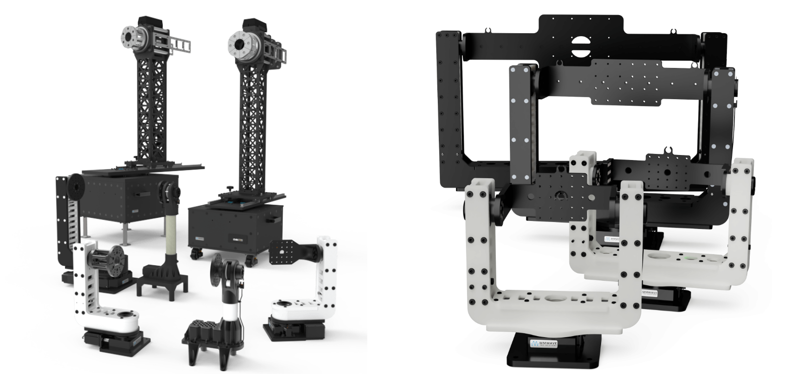
Commercial antenna positioners are built for anechoic chambers. The examples above (roll-over-azimuth and elevation-over-azimuth positioners) are very expensive. They are designed to carry heavy antennas, to repeat a position to a fraction of a degree and to work inside a complete measurement system. That is exactly what a chamber needs, and it is also why they cost far more than a hobby project.
Low-cost alternatives exist in the literature. Olencki et al. from Gdańsk University of Technology describe a mobile far-field system for non-anechoic environments. It is built from in-house rotary heads and an open-hardware VNA, for around 3,630 USD in total [3]. Interestingly, their VNA is also a LibreVNA. Their goal is the same as mine: not to replace a chamber, but to get patterns good enough to check whether a prototype behaves like its simulation model.
My requirements were:
- Two axes, so I can measure full 3D patterns.
- Only dielectric materials near the antenna, so the positioner itself doesn’t become part of the measured pattern.
- Portable: it has to fold and stand on a tripod in the garden.
- Fully automatic: I set it up, press start and come back when it is done.
How does it work?
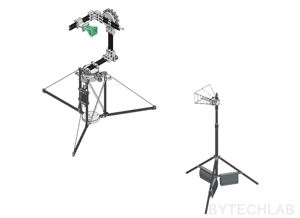
I’m using the Double Ridged Horn Antenna (1–18 GHz) that I have designed as a reference antenna (first VNA port is connected to it). I will publish a post about this antenna soon! The second VNA port is connected to the DUT antenna. The positioner rotates the DUT in two axes to measure the 2D azimuth / elevation cuts and the 3D radiation patterns. Everything is controlled by a Python script on my laptop. I’m using this positioner in my garden.
What the VNA measures is S21, the transmission from port 1 to port 2. For two antennas facing each other in free space, its magnitude follows the Friis transmission equation [1]:
Balanis gives the Friis equation as a power ratio with linear gains. Taking 10·log10 and adding the losses between the VNA and the antennas gives the dB form used here. Realized gain already includes the antenna mismatch.
The reference antenna, the distance and the cables don’t change while the DUT rotates. So every change of |S21| with angle comes from the DUT’s pattern. That is why I plot the patterns normalised to their peak: the shape is right without knowing the cable loss exactly, and even without calibrating the VNA.
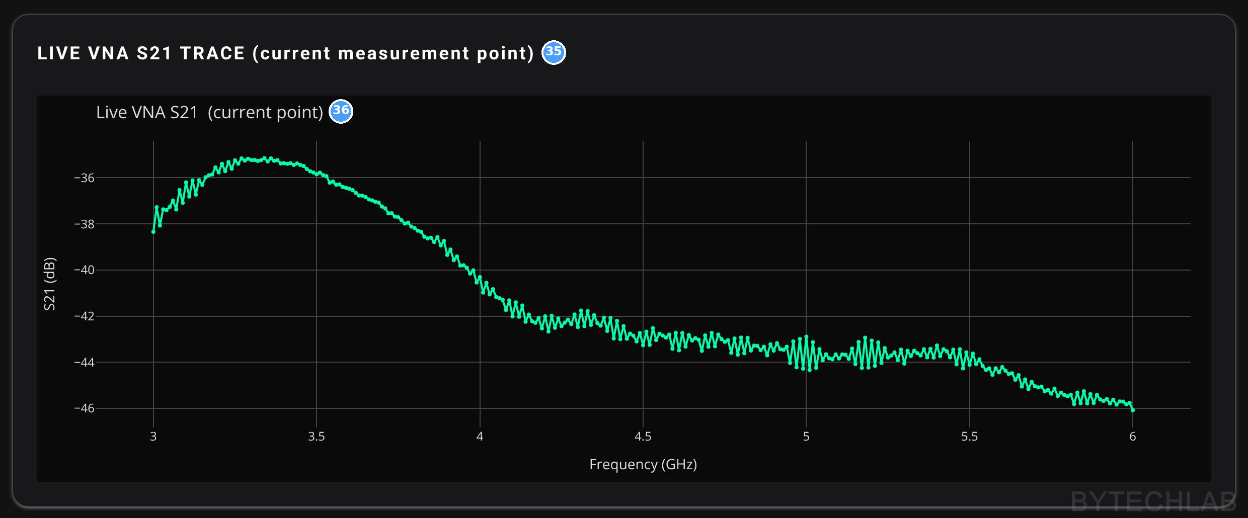
With my numbers, eq. (1) predicts about −24 dB at 4 GHz (11.3 dBi CST realized gain of the reference horn, 12.5 dBi simulated directivity of the PCB horn, R = 1.5 m). At boresight I measured −40 dB, and the gap grows from 14 dB at 3 GHz to 22 dB at 6 GHz. I didn’t calibrate the VNA for these measurements, so this gap contains everything between the two antennas and the VNA: both coax cables, connectors, mismatch and the LibreVNA’s own uncorrected frequency response. For the radiation patterns this doesn’t matter, because all of these stay constant while the DUT rotates and cancel when the pattern is normalised. For an absolute gain I would need at least a thru calibration of the cables, and better a gain-transfer or three-antenna measurement [1], [2].
I have used a Belden H155A00.00B100 low loss cable, it was low loss enough (and quite cheap) to solve my cable loss / VNA dynamic range issue. The cable is quite long 2 x 5 meters so every dB of loss matters. I didn’t want to buy extremely expensive low loss cable either, that’s why I have picked something in between.
How far is far enough?
A radiation pattern is defined in the far field, where the incoming wave is (almost) a plane wave. The usual criterion is [1], [2]:
Here D is the largest dimension of the antenna. The PCB horn’s aperture is 100 × 99.5 mm , so D ≈ 141 mm. That puts 2D²/λ at 0.80 m at 6 GHz and 0.93 m at 7 GHz, so 1.5 m is comfortably beyond it.
The criterion is really a limit on the phase error across the aperture. A spherical wave from a source at distance R reaches the edge of the aperture slightly later than its centre. The maximum phase difference is:
At R = 2D²/λ this gives exactly 22.5° (π/8), which is the error the classic criterion accepts [1], [2]. For the PCB horn at 1.5 m it is 6° at 3 GHz and 12° at 6 GHz. According to IEEE 149, the visible effect of such a phase error is that pattern nulls get partially filled and sidelobe levels change [2], so it matters most for the deep nulls.
The reference horn is the weak point. It is much larger, with D ≈ 281 mm across the aperture. For the pattern, what counts is the curvature of the wave that arrives at the DUT, and IEEE 149 treats it as a spherical wave from the reference antenna [2], which is exactly what eq. (3) describes. Balanis states that the Friis equation needs R > 2D²/λ with D the largest dimension of either antenna [1]. For the reference horn that is 1.6 m at 3 GHz and 3.2 m at 6 GHz, so the prediction from eq. (1) is only a rough check at the upper frequencies.
I might get better results when I will move two antennas further apart, this is problematic due to libreVNA limited dynamic range and cable loss. I have purchased a new VNA though, so I will probably try this in the future.
The ground echo
Without absorbers, the biggest unwanted signal is the reflection from the ground between the antennas. The ground acts like a mirror.
The signal reflected form the ground and other objects (like building, trees etc.) travels longer than signal that hits the antenna directly, so this echo could be removed with time gating [2]. Olencki et al. do exactly that with their LibreVNA [3]. My software doesn’t do it yet, because it stores only |S21| in dB and throws away the phase. I will try to implement this method in the future.
2) MCAD & ECAD design
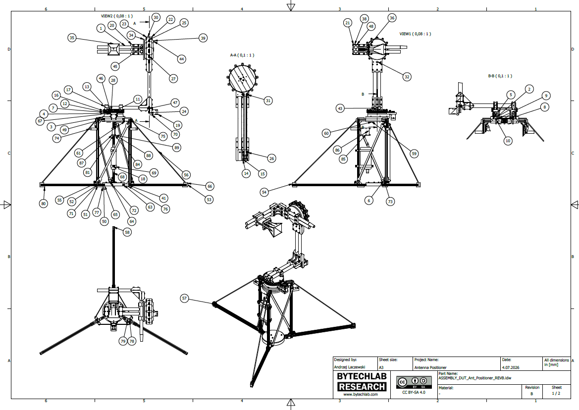
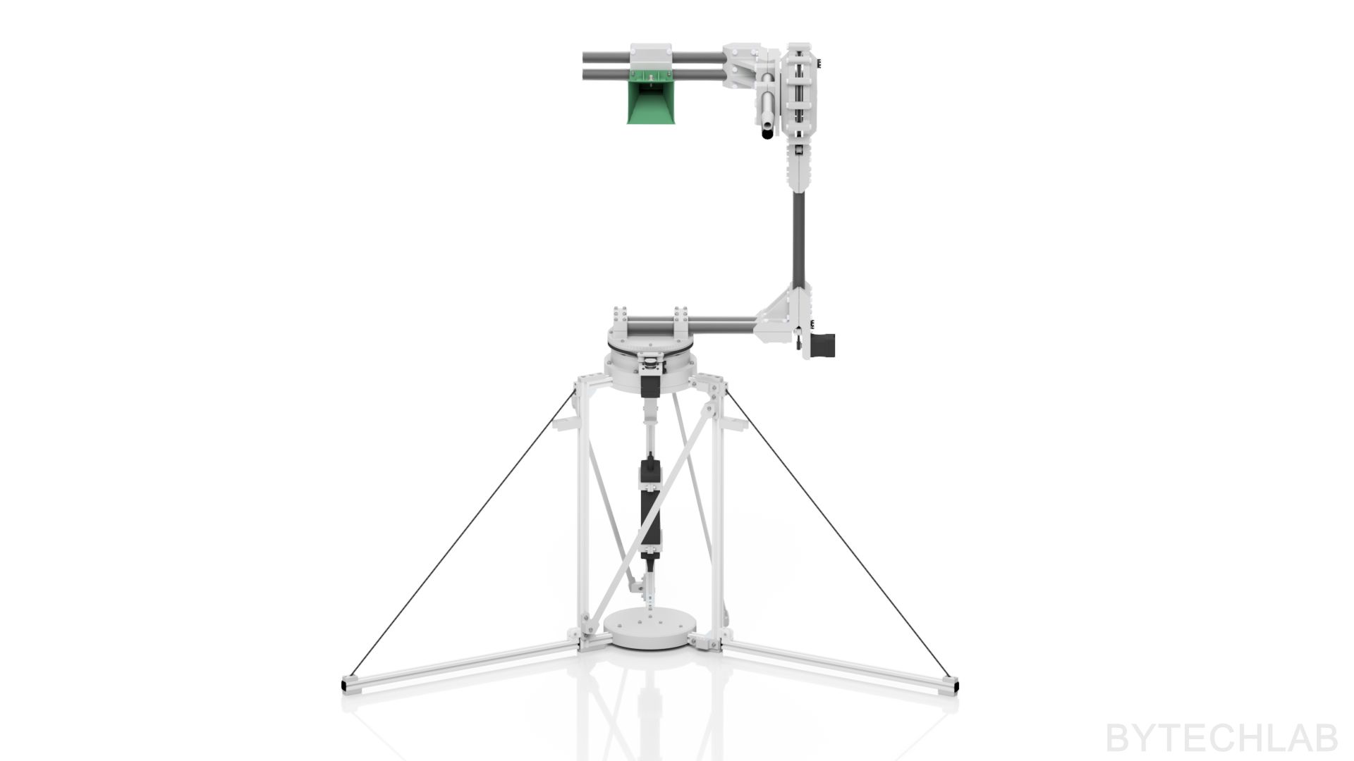
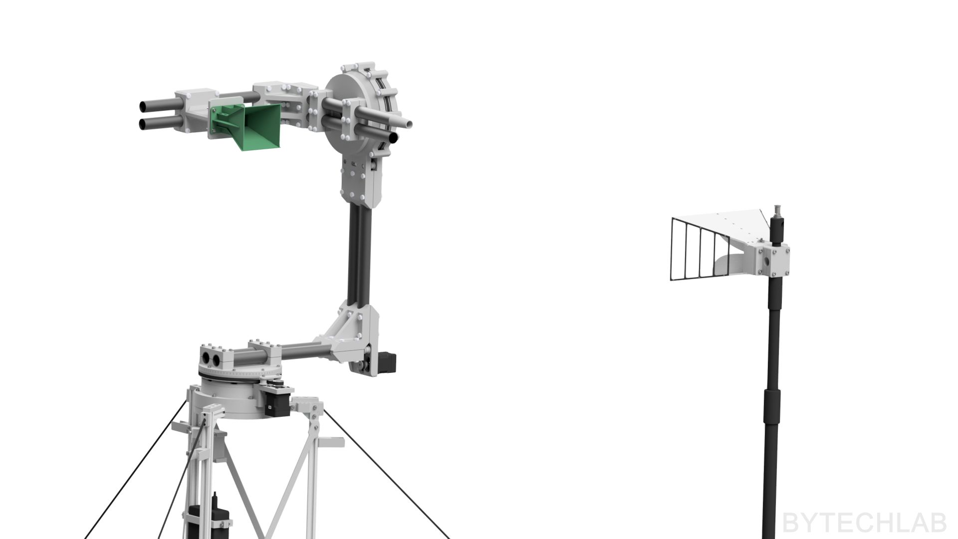
The whole positioner is designed in Autodesk Inventor. It is an elevation-over-azimuth positioner. The lower A axis rotates everything above it (azimuth). The upper B axis tilts the antenna boom around a horizontal axis (elevation). With azimuth −180…+175° and elevation −90…+90°, the two axes cover the full sphere.
Most parts are 3D printed in PLA. The COTS parts are mostly standard:
- 20 × 20 mm aluminium profiles for the lower frame
- Eight 27 × 24 mm fiberglass tubes for the arms
- HTD3M timing belts and pulleys
- a large 6020-2RS bearing (150 × 100 × 24 mm) in the azimuth joint
- two 6016 POM bearings (125 × 80 × 22 mm) in the elevation joint
- a lot of M6 × 50 nylon screws with nylon nuts
The full BOM is in the GitHub repository.
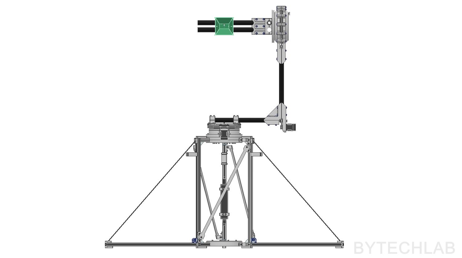
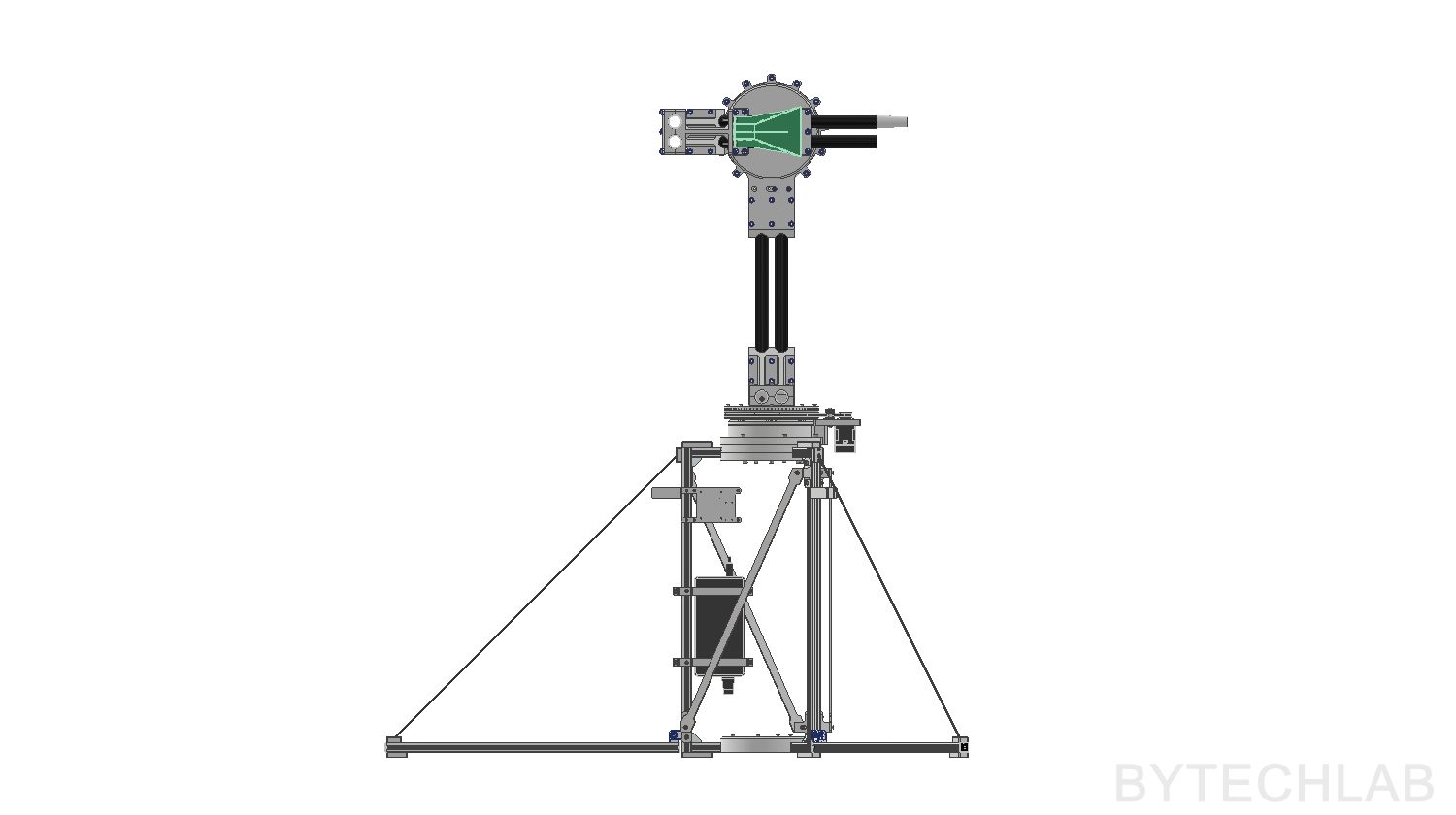
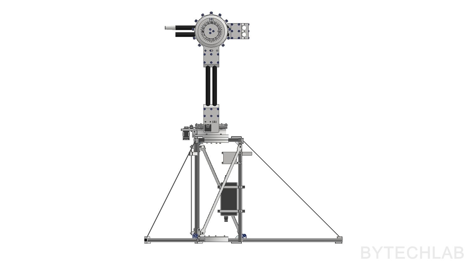
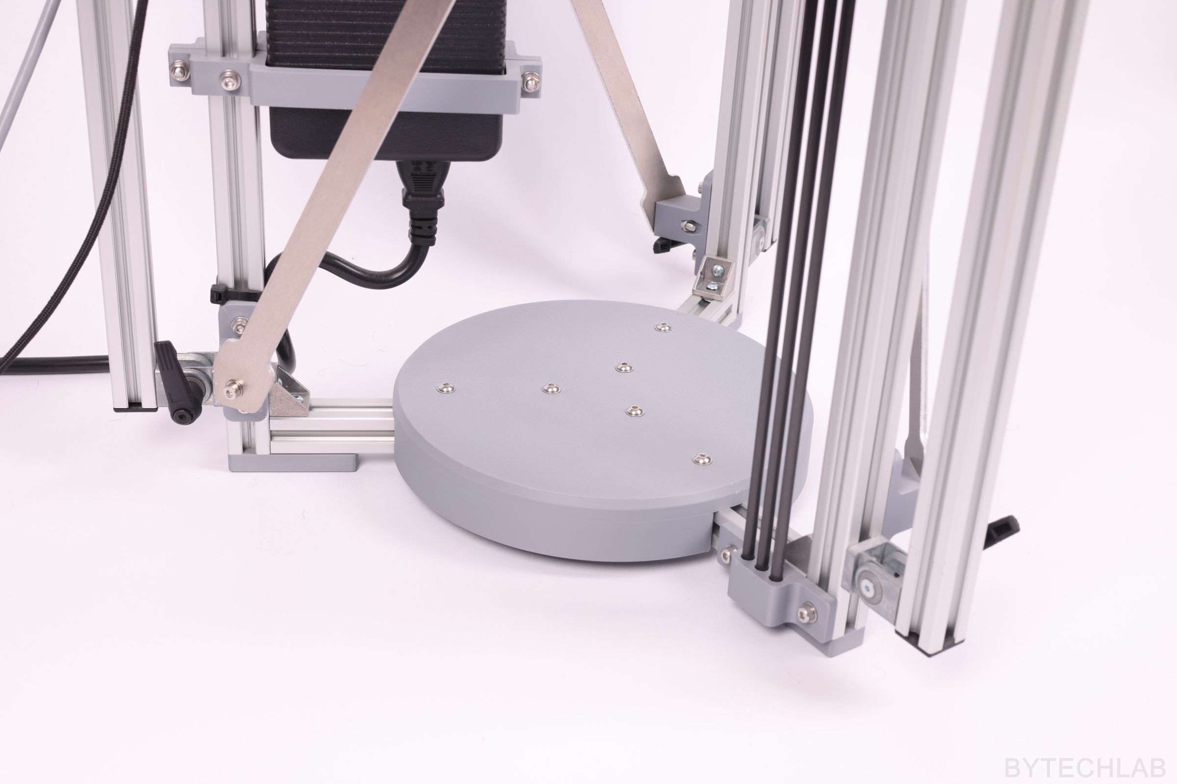
The front view shows the main idea of the layout. The lower half is allowed to contain metal: the frame with three foldable legs, the azimuth motor, the power supply and the electronics. The upper half, everything that the DUT “sees” at short distance, is made of dielectric materials.
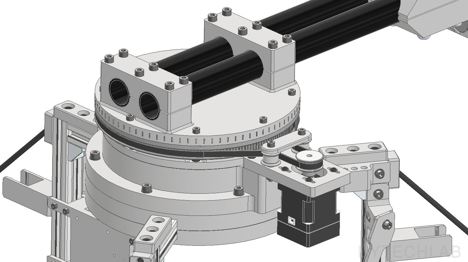
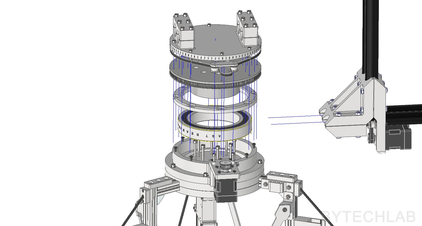
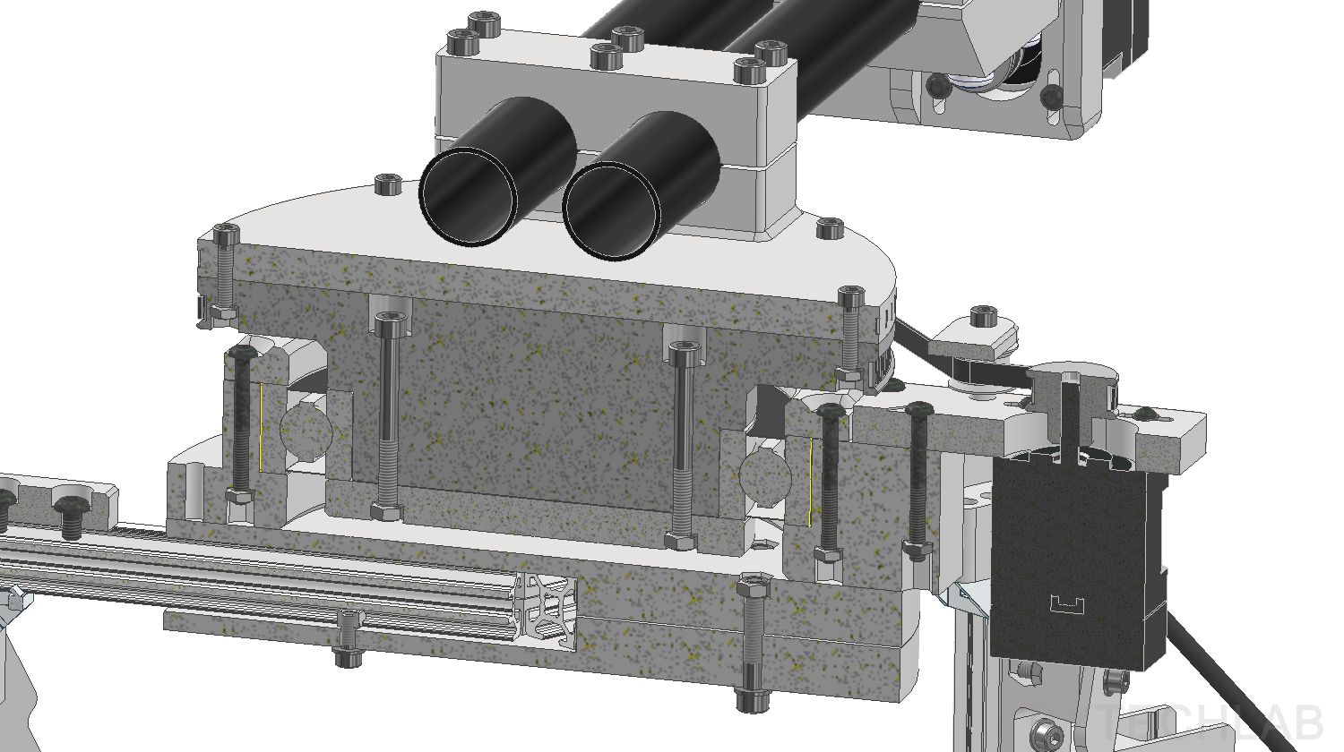
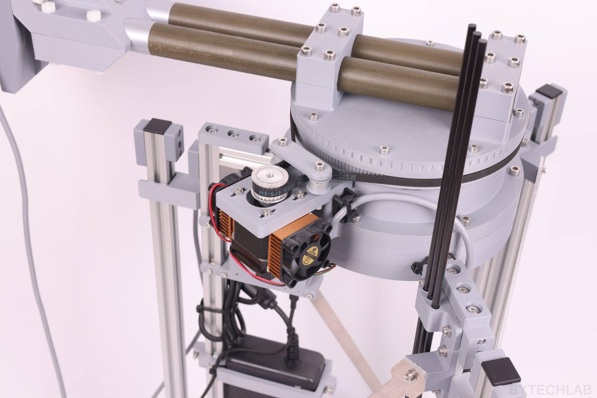
The azimuth (A) joint carries the whole upper structure. A 6020-2RS bearing takes the load, and a printed rotating stage sits on top of it. The motor drives the stage through an HTD3M belt: 24 teeth on the motor pulley and 192 teeth on the stage, a ratio of 8. Two printed idlers with small bearings keep the belt wrapped around the big pulley.
The belt reduction gives more torque at the output, a finer step and no gearbox backlash. One encoder count of the motor is 0.0027° at the antenna after the 8:1 gearbox, far finer than the measurement needs. The MKS manual gives an axis error of about ±15 encoder counts in the absolute-move mode [4], which is only 0.04° at the antenna. So the real pointing accuracy is set by belt stretch and the stiffness of the printed parts.
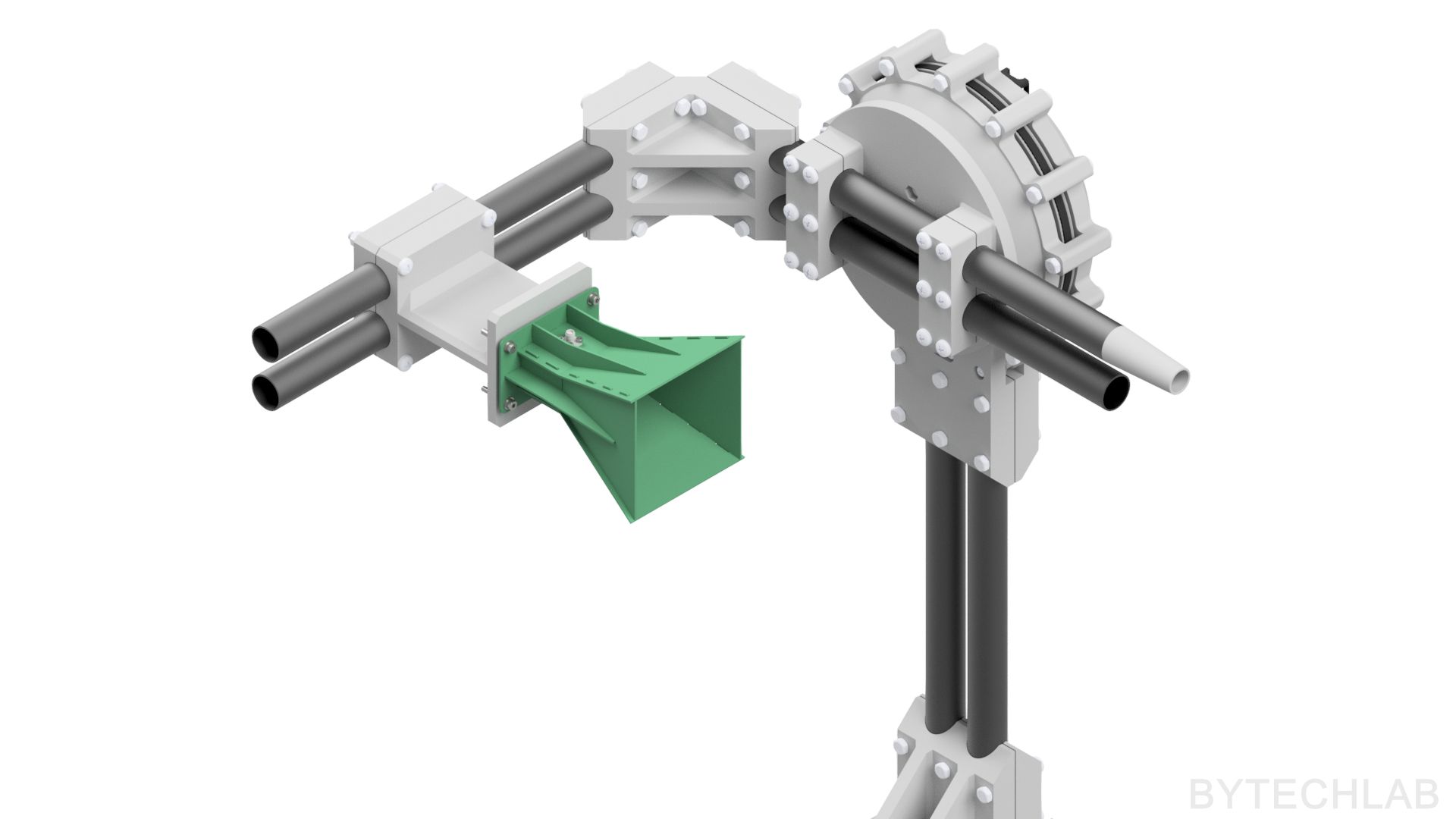
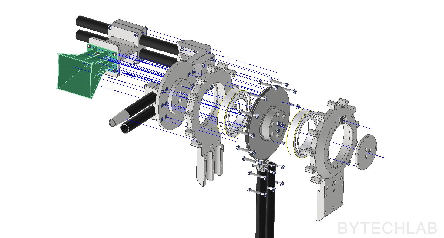
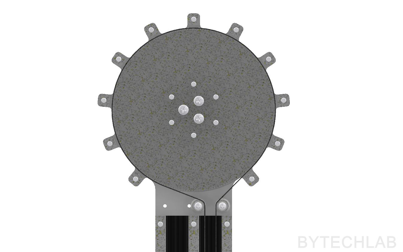
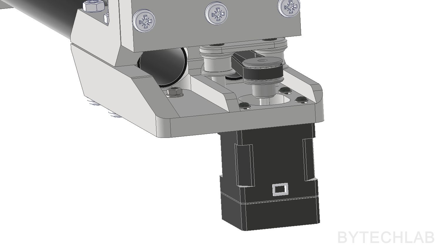
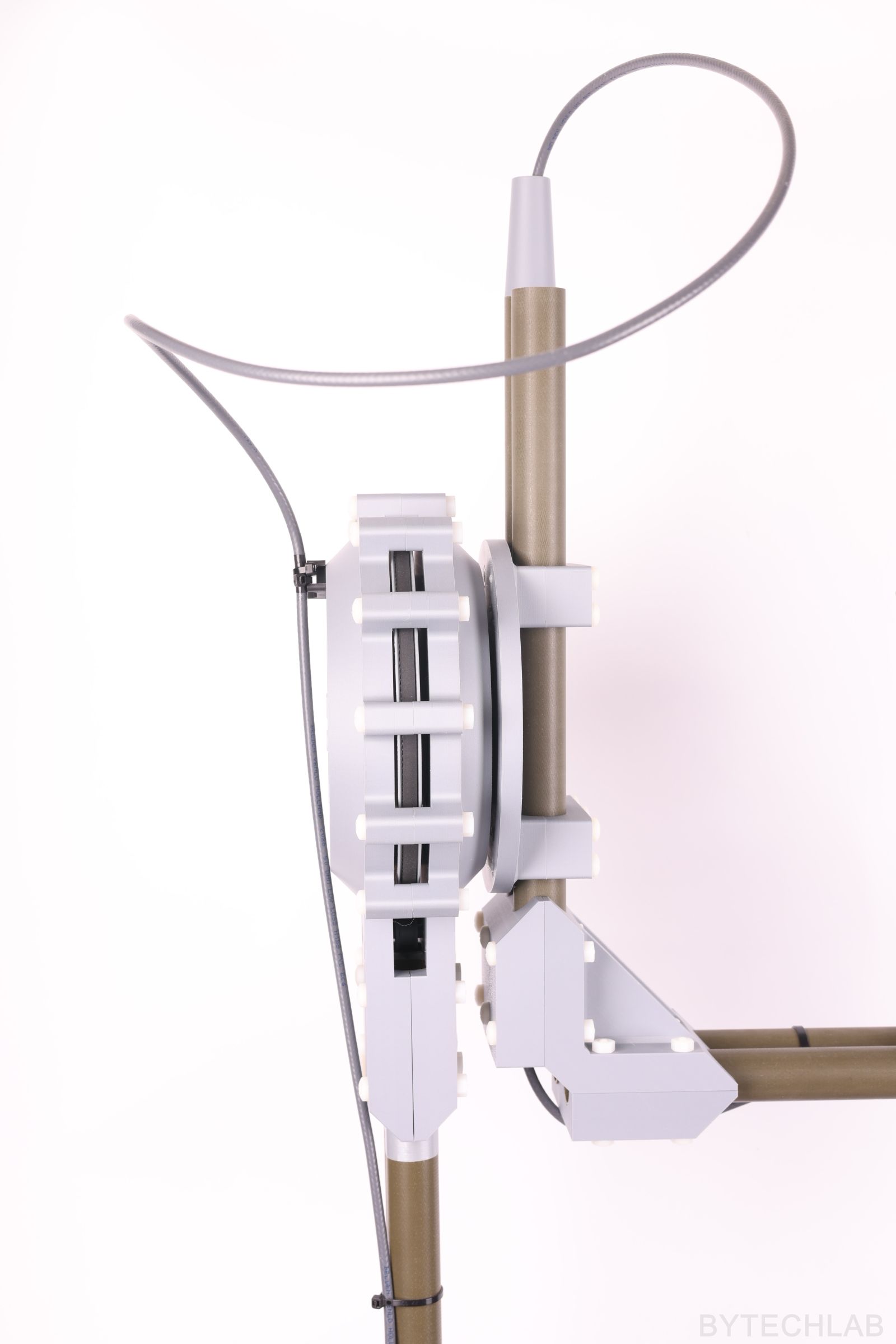
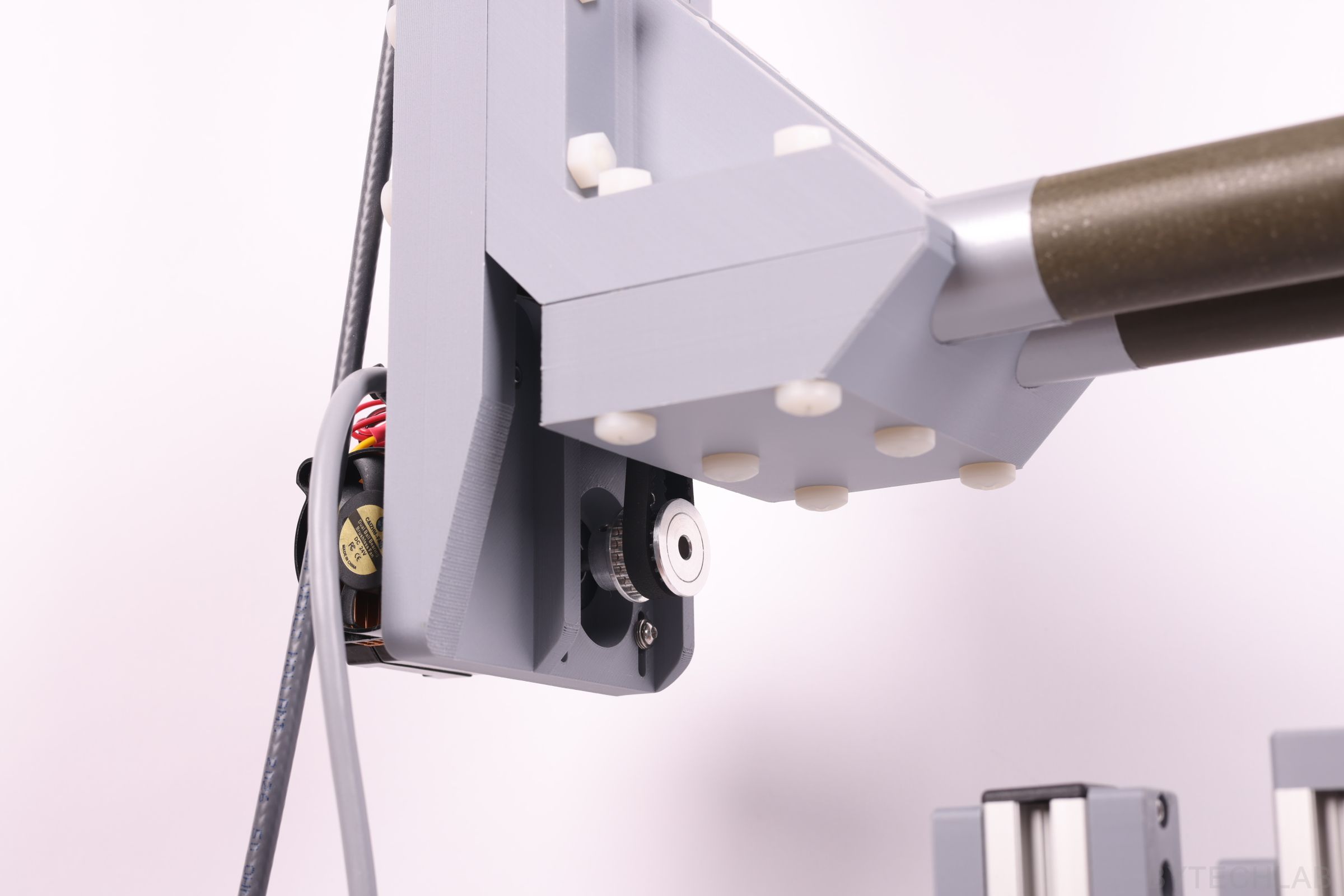
The elevation (B) joint is the most interesting part mechanically. It sits right next to the DUT, so it can’t contain a motor. Instead, the B motor is mounted low, on the bracket next to the azimuth stage. It drives the B axis through a 1530 mm long HTD3M belt that runs up inside the fiberglass pipe to a printed 200-tooth pulley (20 teeth on the motor, ratio 10).
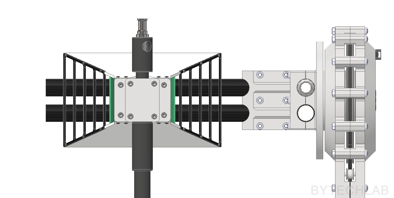
The B axis turns in two 6016 POM bearings (all-plastic ball bearings), and the belt idlers next to it use 604H ceramic ball bearings. Every screw in this area is nylon, and the antenna boom is a pair of fiberglass tubes held by 3D printed PLA clamps.
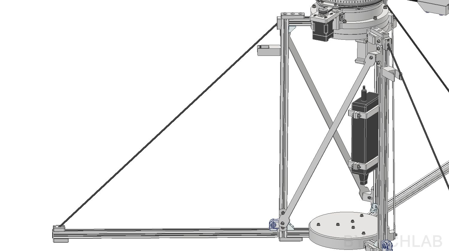
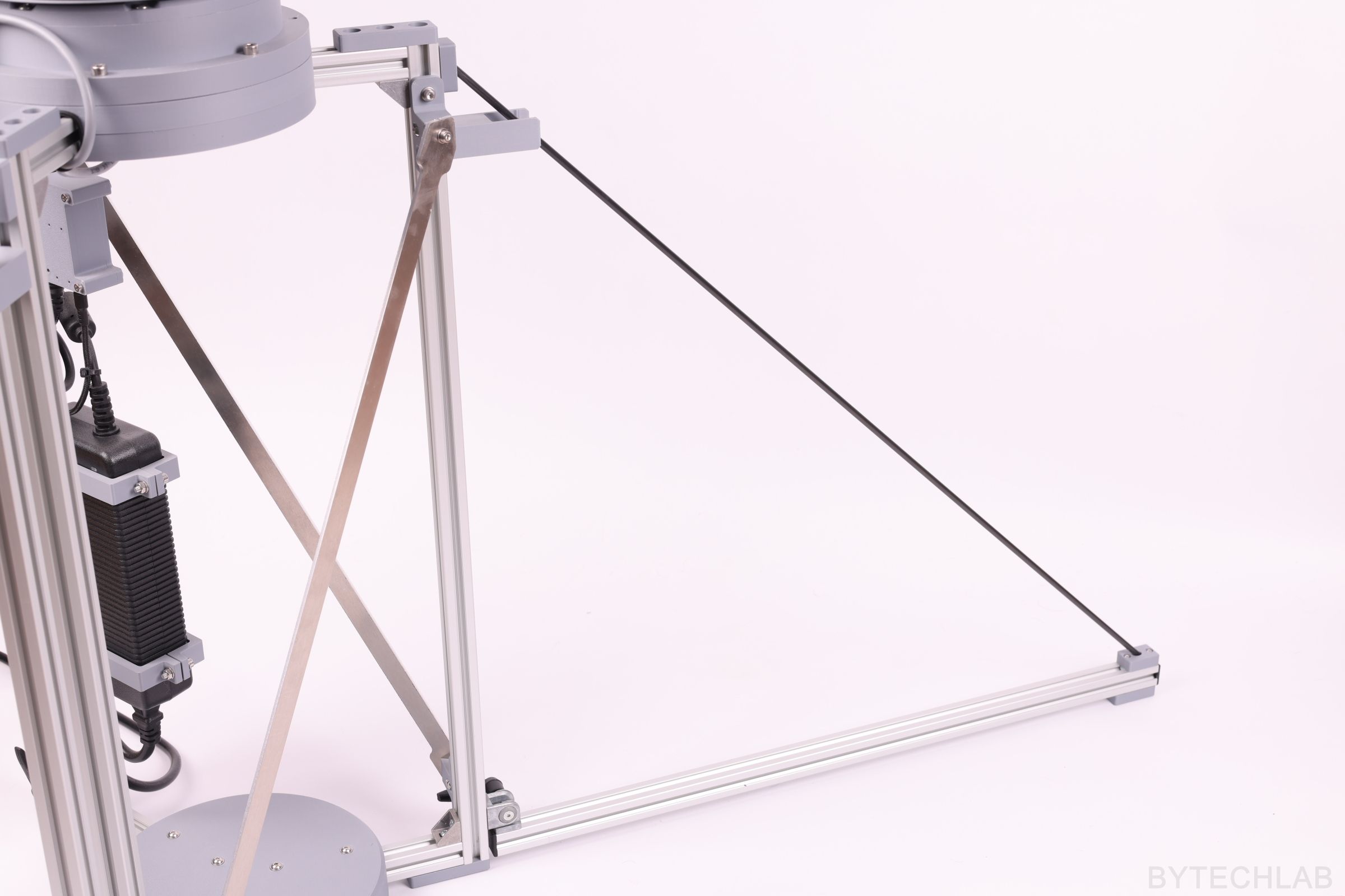
The lower frame is made of 20 × 20 mm aluminium profiles. The three legs fold up for transport on hinges and latch into printed holders. Three 5 mm carbon rods carry the load to three legs.
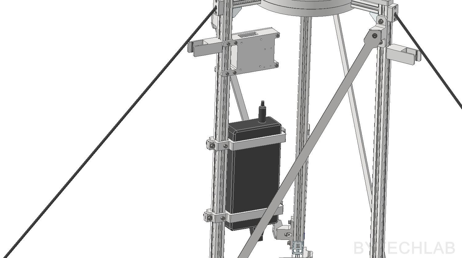
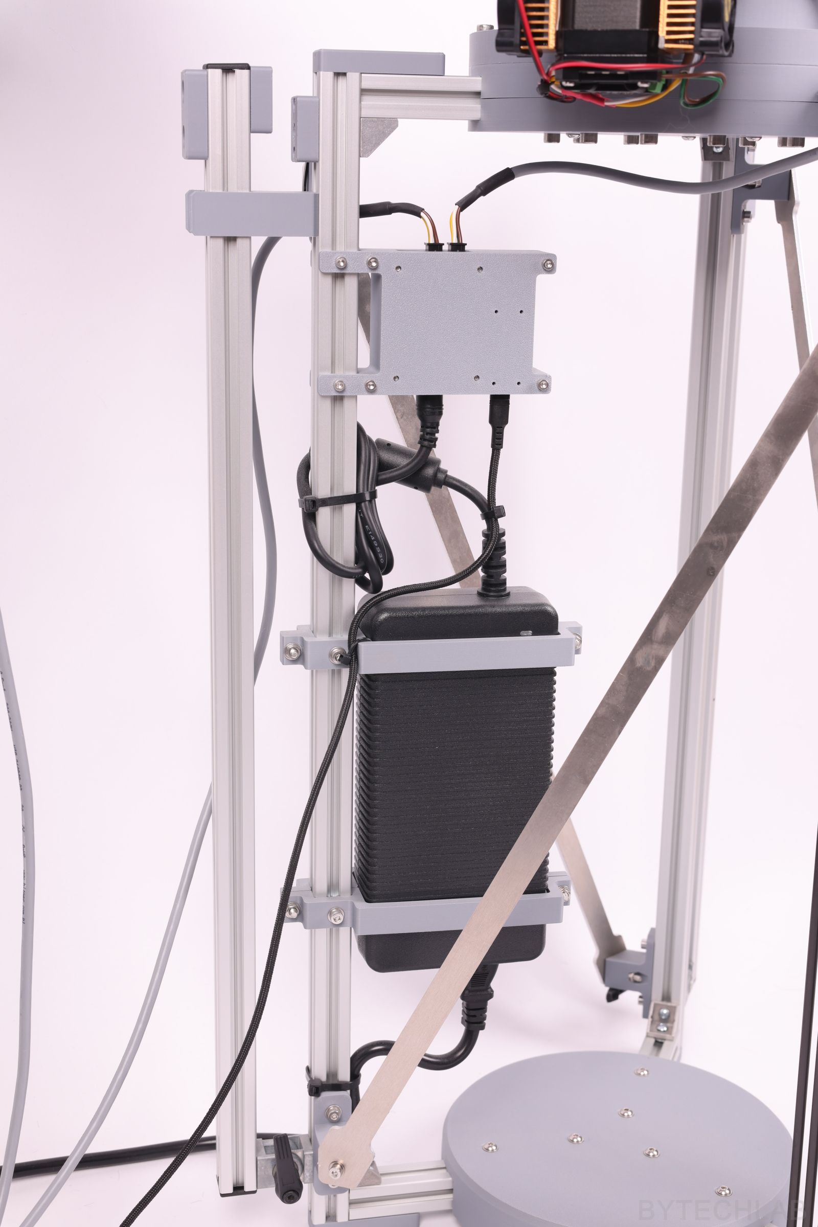
A 24 V power brick is held on the frame by four printed clamps. A small printed box above it holds the MKS CANable V2.0 adapter. There are only two USB cables connected to the laptop: one from the CANable and one from the LibreVNA.
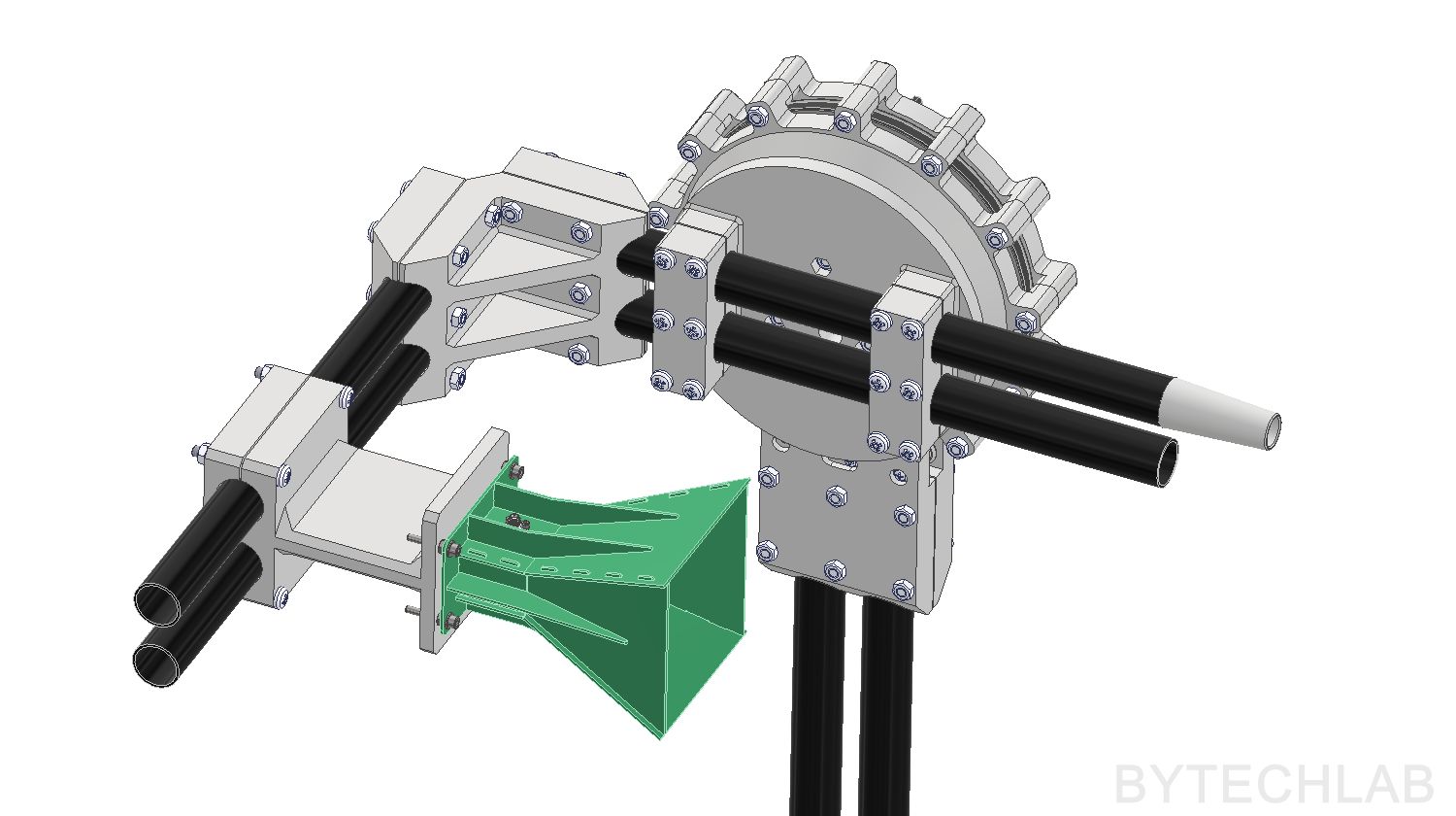
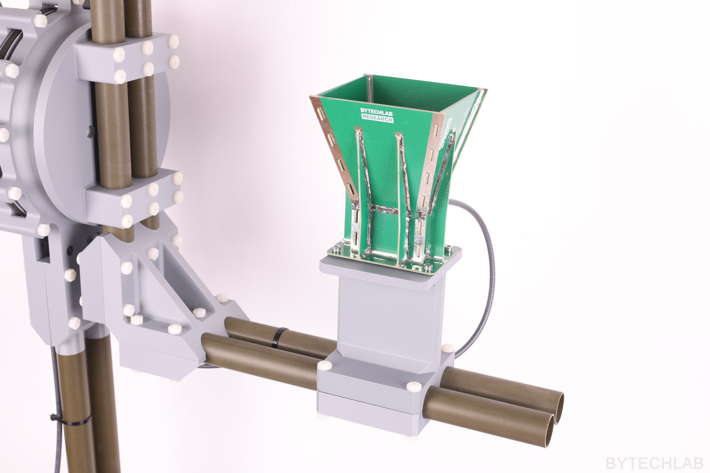
The DUT mount is the only part that changes between antennas. The PCB horn sits in a dedicated 3D printed mount on the fiberglass boom, which puts its aperture at the right place relative to the axes. For another antenna I only need to print a new mount. The CAD library in the repository already contains models of my other antennas, which I use to check the fit before printing.
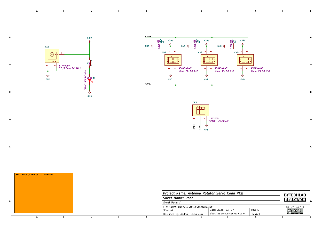
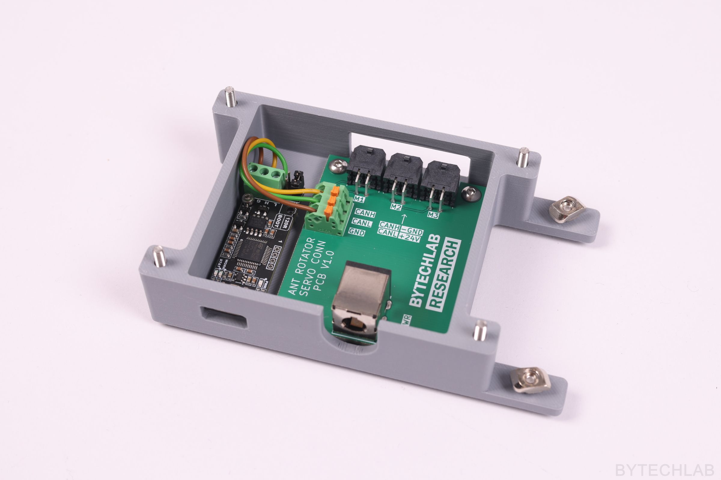
I have designed a simple PCB just to connect all of the servo motors together (using nice Molex connectors). I’m using MKS SERVO42D 40 CAN MT closed-loop motors, controlled via CAN bus by the CANable V2.0 USB ↔ CAN converter.
The PCB is deliberately simple:
- a 5.5/2.5 mm DC jack for 24 V and a power LED
- three Molex Micro-Fit 3.0 2 × 2 connectors, one per motor (24 V, GND, CANH, CANL), each with a 10 µF decoupling capacitor
- a 3-pin terminal for the CAN lines from the CANable
Two connectors are used today. The third is a spare for a future third axis.
In the GitHub repository (MCAD folder) you can find the following files:
- Autodesk Inventor project of the antenna positioner,
- exported STL files for 3D printing,
- exported STEP file of the whole assembly,
- exported PDF file with the assembly drawing, BOM and assembly instructions,
- exported assembly renders.
In the GitHub repository (ECAD folder) you can find the following files:
- KiCad project of the antenna positioner PCB,
- exported Gerber files for manufacturing,
- exported STEP file of the PCB,
- exported PDF file with the schematic and layout.
In the GitHub repository (SOFTWARE folder) you can find the following files:
- ANTENNA_POSITIONER.py, libreVNA.py and install_packages.bat,
- example measurement results (CSV, notes, plots, 3D HTML),
- 10_MEAS_VS_SIM_COMPARISON.py with the CST far-field exports.
3) EM simulations
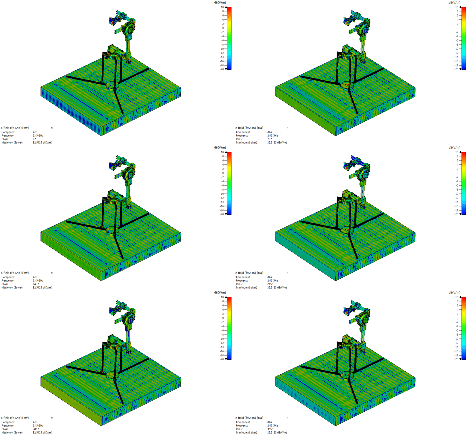
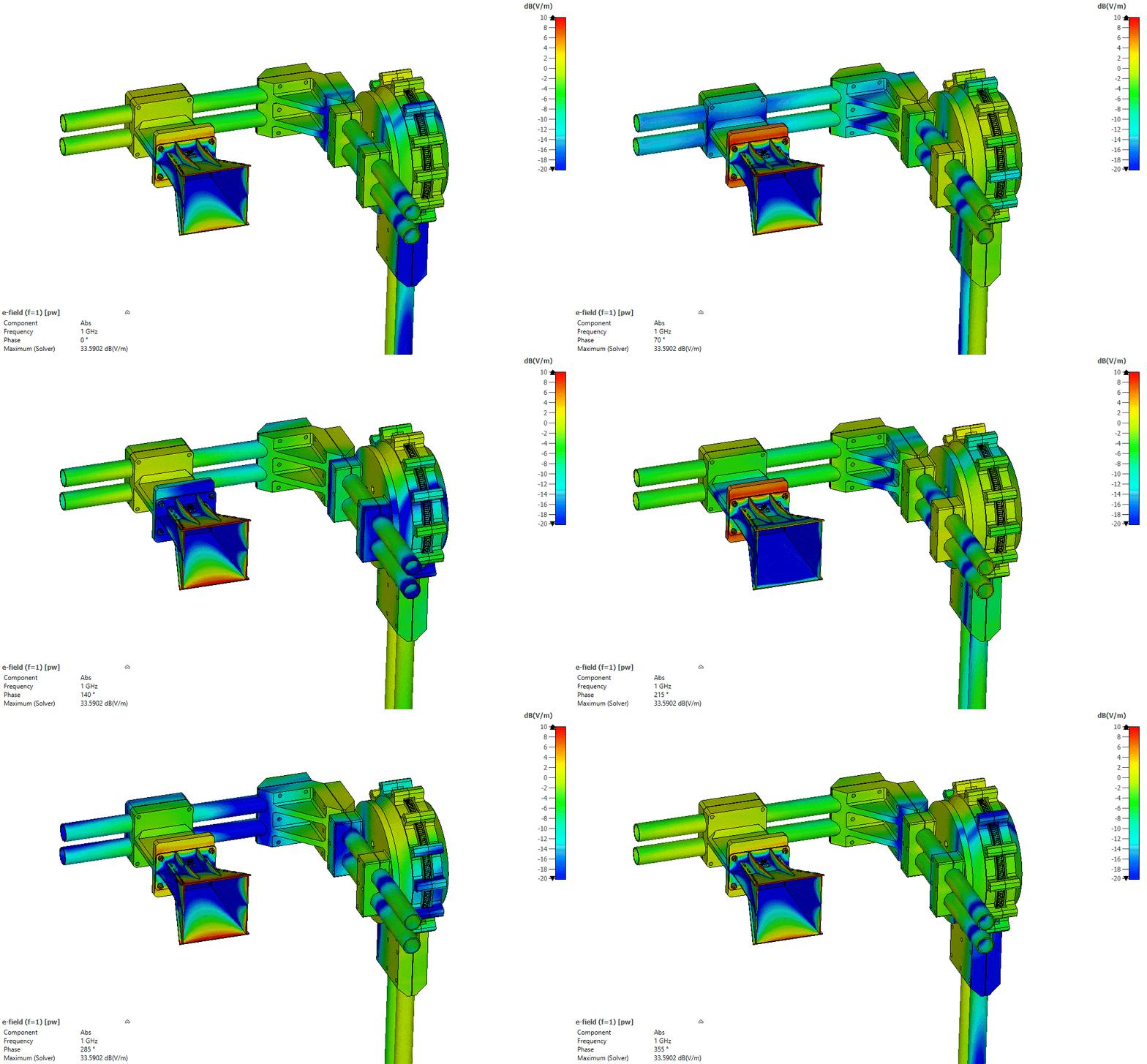
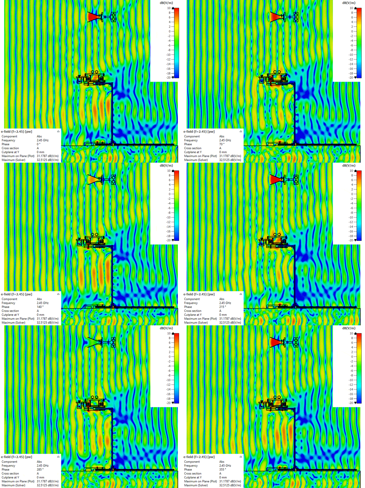
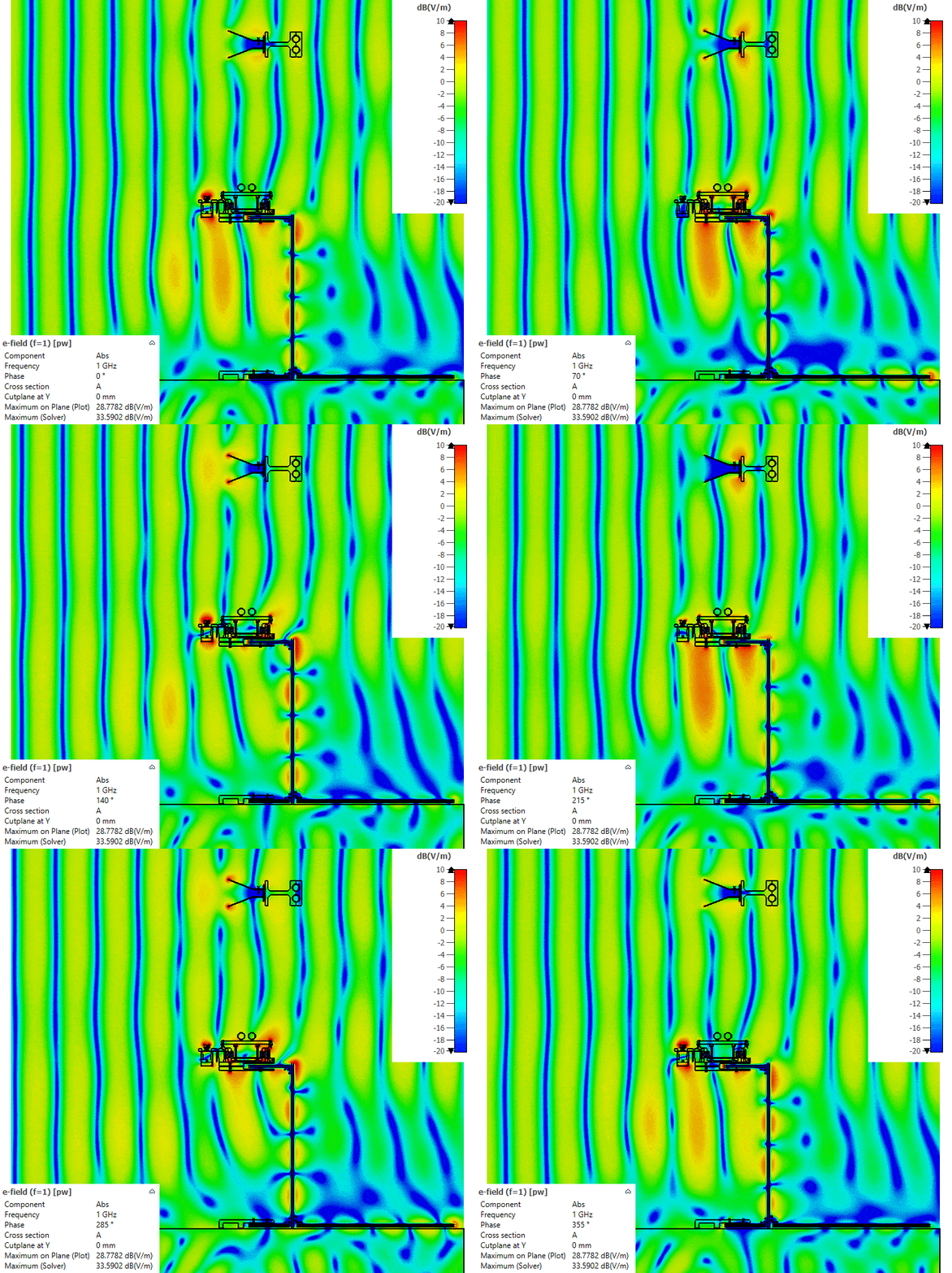
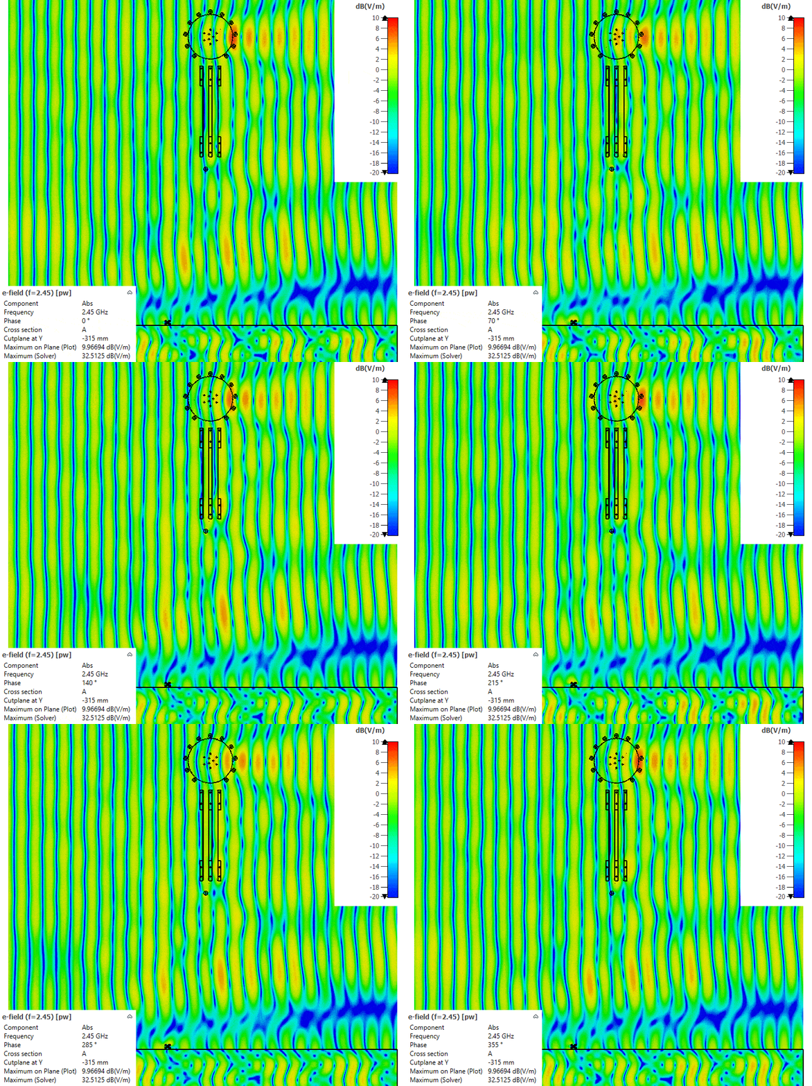
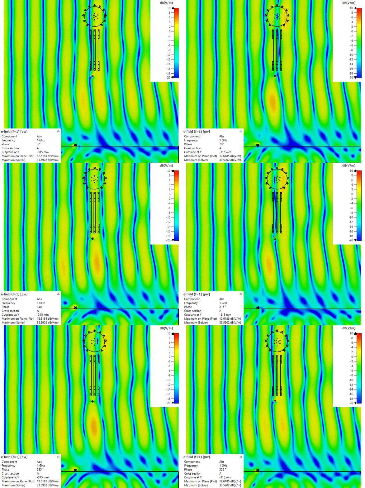
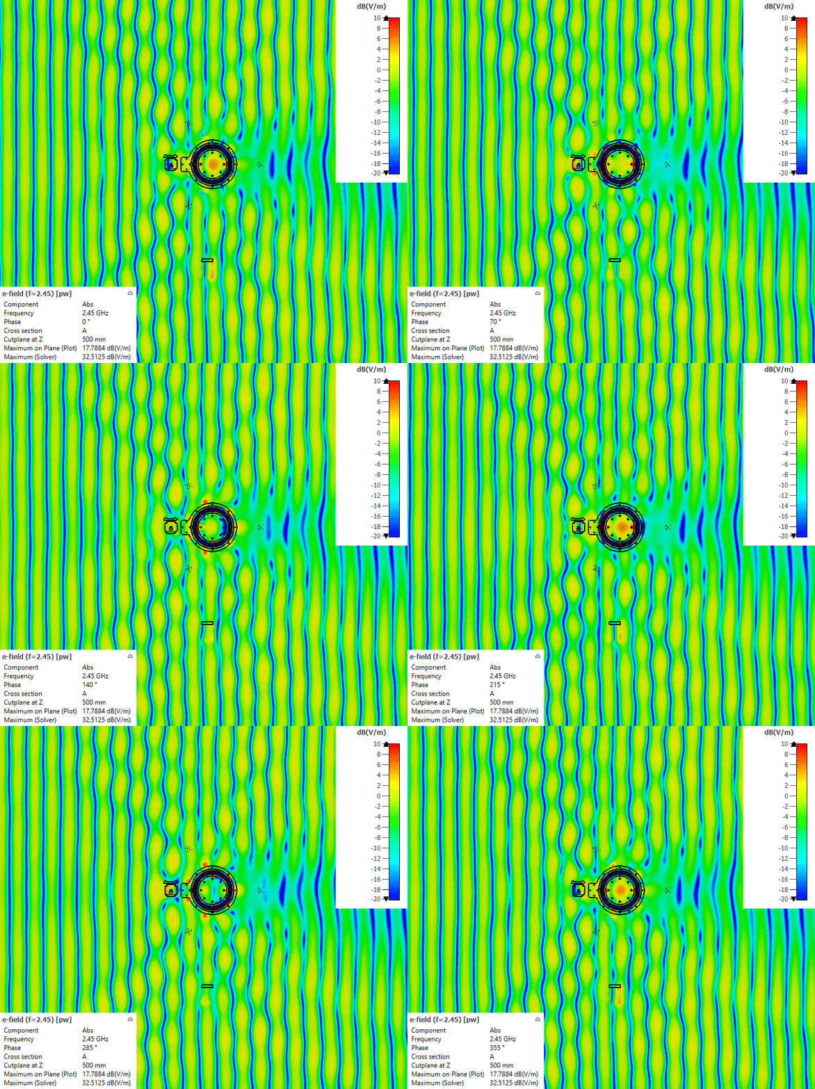
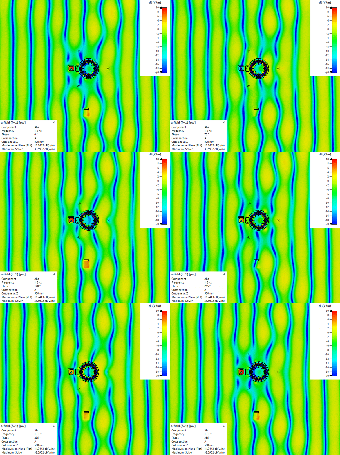
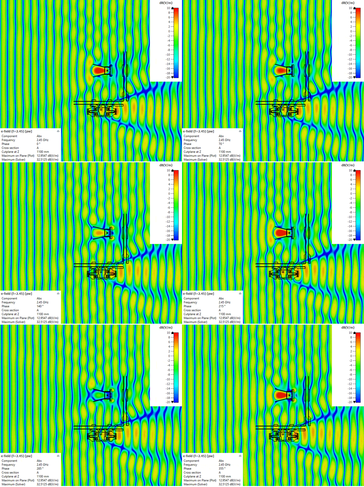
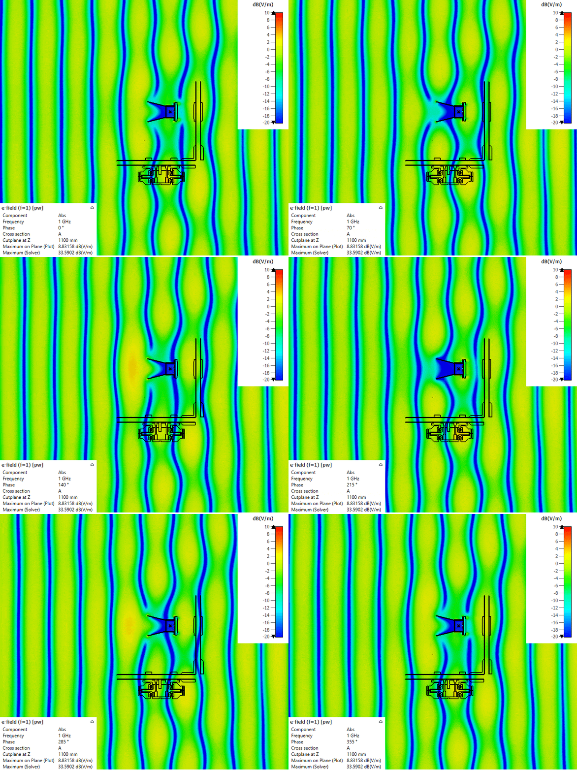
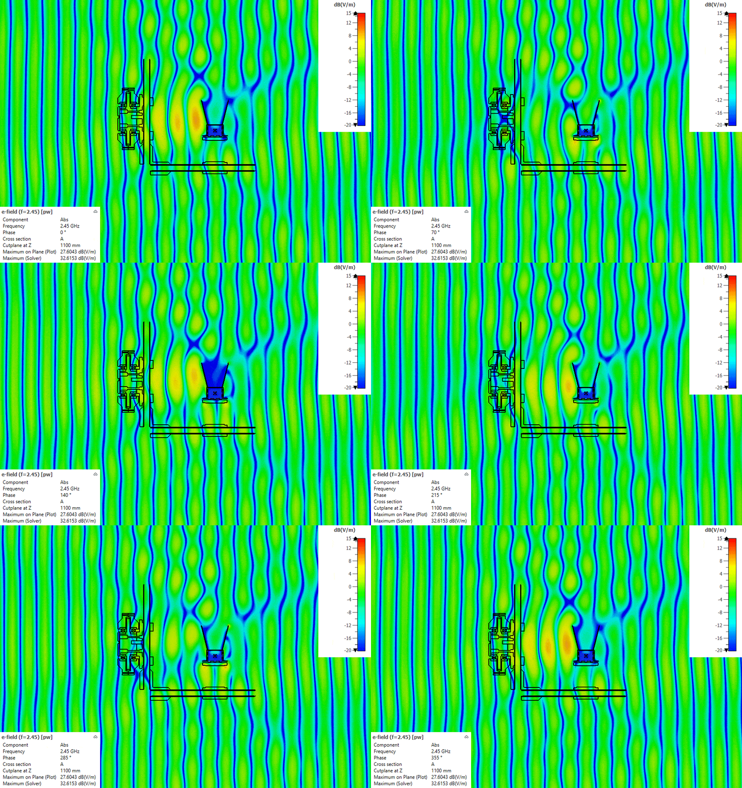
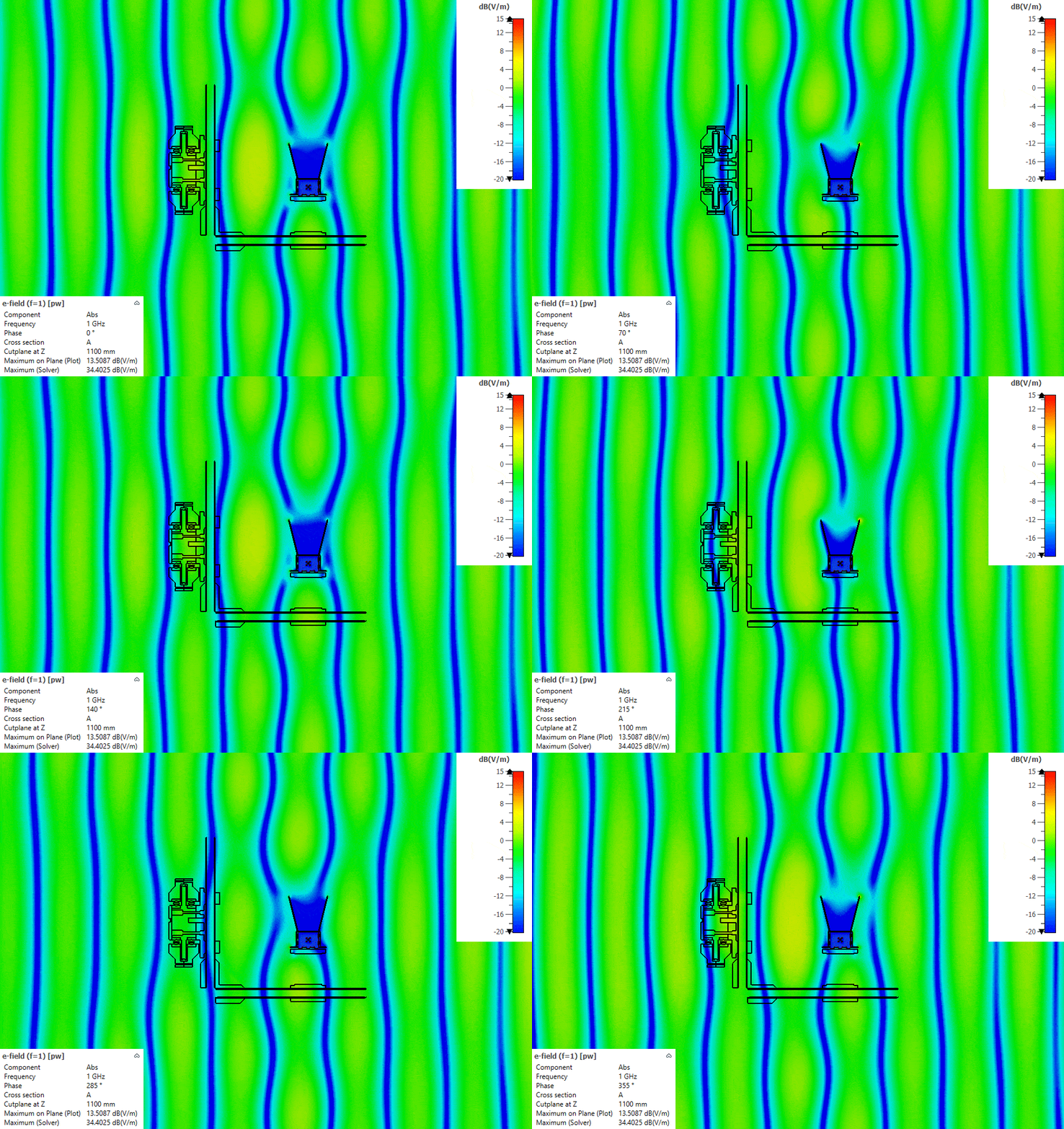
I have made these simple simulations of the whole antenna positioner placed on the ground and illuminated by a plane wave (1 or 2.45 GHz), just to check how the construction alters the wavefront. Unfortunately, I was able to simulate only these two frequencies due to the mesh size.
The simulations were done in CST Studio Suite with the time-domain solver. A plane wave arriving from the boresight or side direction illuminates the positioner standing on a block of ground. The field plots show the E-field magnitude in dB in vertical and horizontal cuts through the A and B joints. Ideally, the straight stripes of the plane wavefronts would pass through the antenna position undisturbed. Where the structure scatters, the stripes bend. You can see a lot of interesting electromagnetic effects on these animations !
The model is large in wavelengths. The positioner is about 1.35 m tall, which is 4.5 λ at 1 GHz and 11 λ at 2.45 GHz. A mesh fine enough for 3–6 GHz, where I actually measure, would be far too big for my PC. These simulations are not simulations of the measurement itself (there is no reference antenna and no DUT), but they show where to expect trouble.
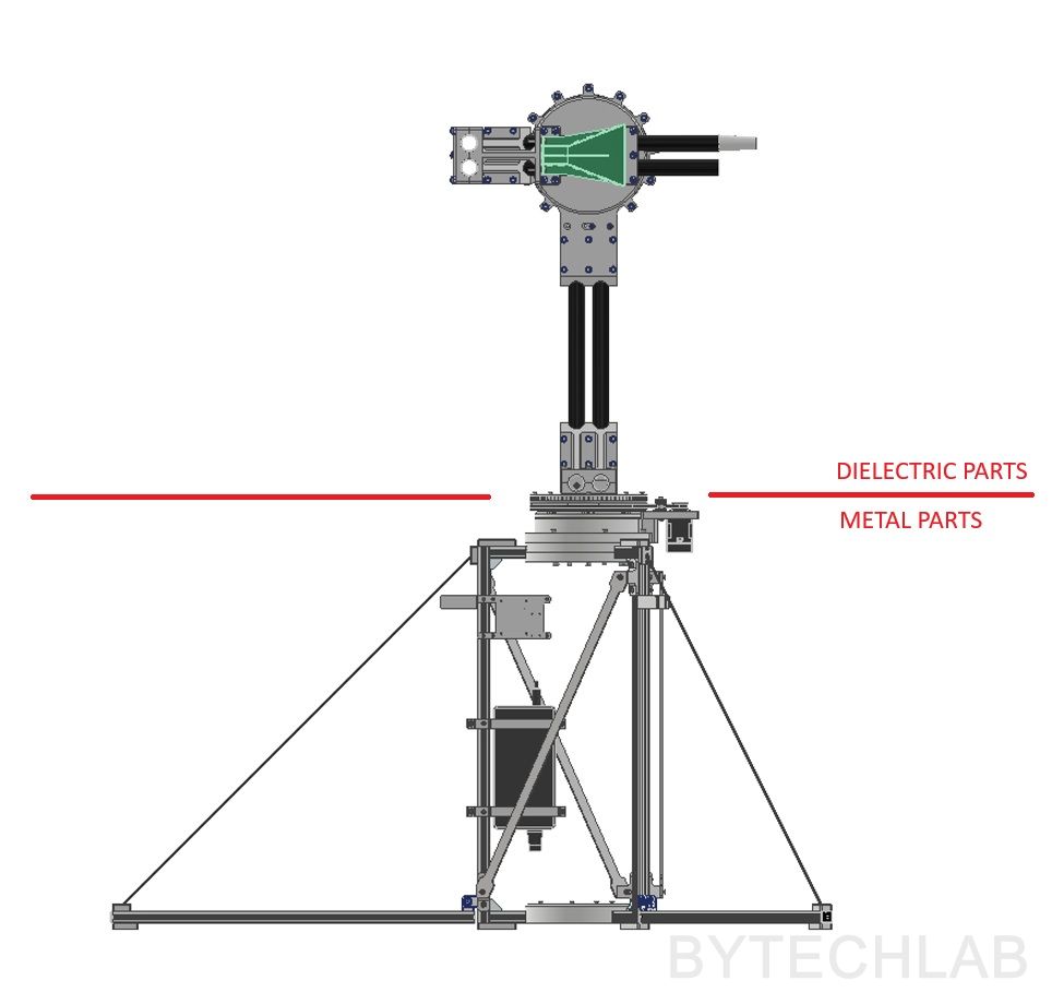
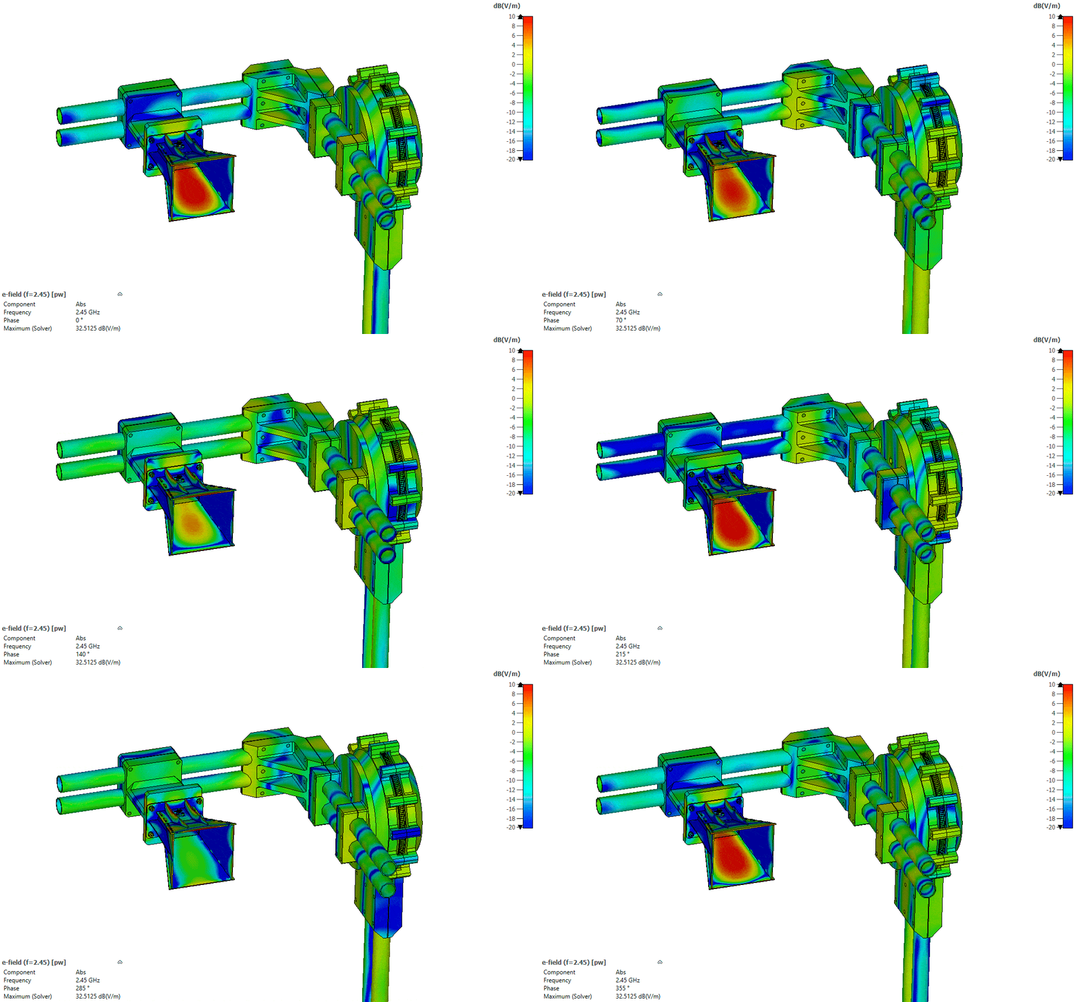
The upper section of the positioner is made from dielectric materials only, to minimise the impact on the wavefront. The bearings are either ceramic or plastic, the pipes are made from fiberglass composite, the screws are nylon and the rest is 3D printed from PLA with low infill, both to reduce the effective permittivity and the weight.
The plots confirm the split. The strongest disturbance comes from the metal in the lower half (aluminium frame, motors, power supply) and from the ground itself. Around the DUT and the antenna boom, the wavefronts stay almost straight (boresight wavefront direction). The dielectric parts of the B joint affect the wavefront a little (side wavefornt direction – B joint overshadows DUT) – this shouldn’t be a big problem for directional antennas (10 dBi +), the side lobes might be a little asymmetric due to this. The only way to check how it really works is to build it and measure some radiation patterns !
4) Software
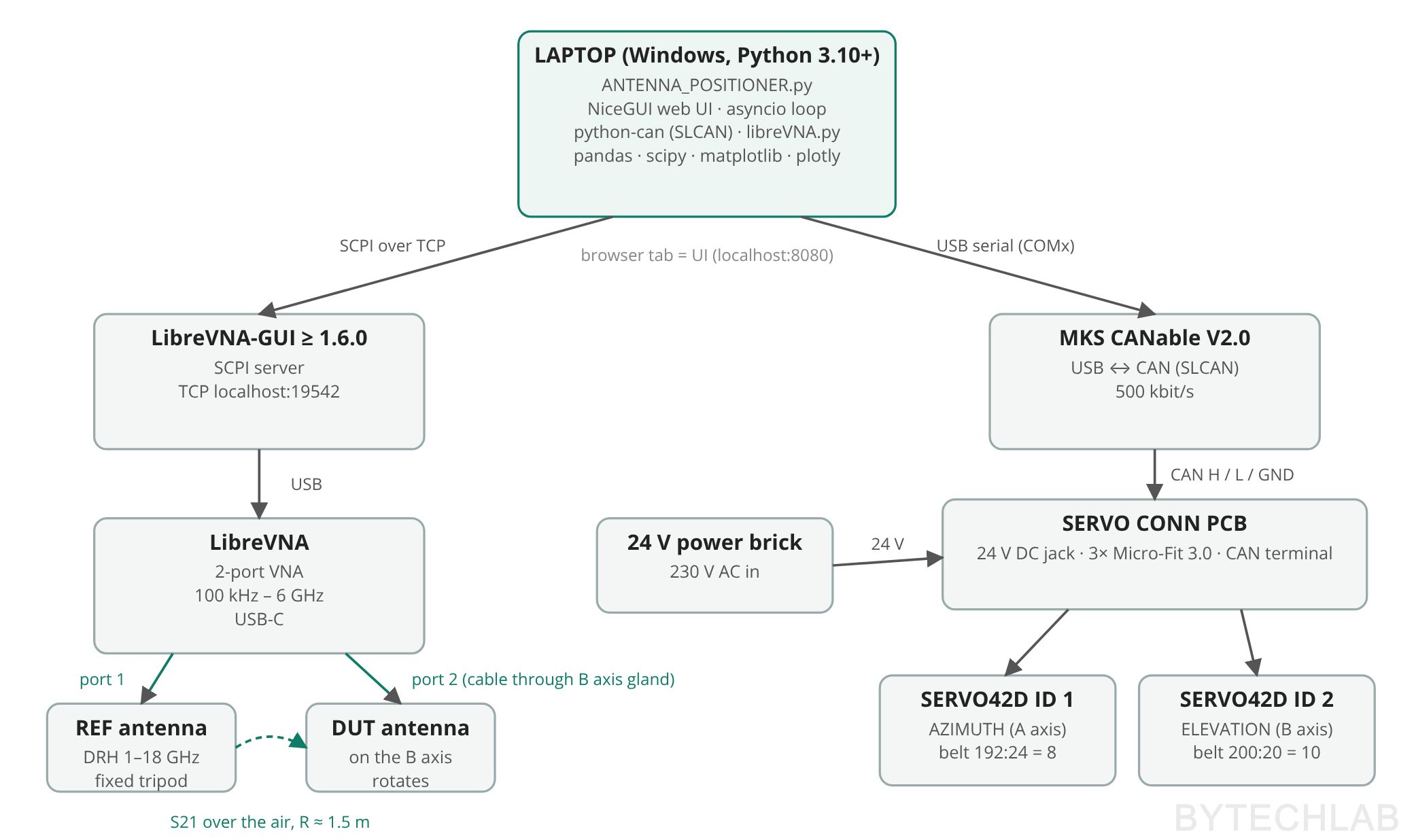
The software is a single Python program, ANTENNA_POSITIONER.py (about 3,000 lines). It runs on my Windows laptop with Python 3.10+, and install_packages.bat installs everything it needs. The user interface is a web page served by NiceGUI and opened automatically in the browser, so the GUI is really a local website on localhost:8080. Everything runs in one asyncio event loop: button handlers, motor moves and VNA sweeps.
The laptop talks to two devices. The motors are on a CAN bus behind the CANable adapter, which python-can drives with the SLCAN protocol at 500 kbit/s (the motors’ default CAN rate [4]). The VNA is controlled through LibreVNA-GUI, which must be running: it has an SCPI server on a TCP port set in its preferences (19542 on my laptop), and the script sends text commands to it [5].
| Library | Used for |
|---|---|
| NiceGUI | The whole user interface: a web page served on localhost:8080 |
| python-can + pyserial | CAN bus over the CANable V2.0 USB <-> CAN dapter |
| libreVNA.py [5] | Small socket helper from the LibreVNA project: sends SCPI commands, reads answers, parses the trace data |
| asyncio + ThreadPoolExecutor | One event loop for UI and measurement. |
| NumPy, pandas | Angle grids, data storage, CSV export, normalisation |
| SciPy | Savitzky–Golay filter over frequency, Gaussian smoothing of the preview |
| Matplotlib | PNG polar and 1D plots after the measurement (Agg backend, no window) |
| Plotly | Live preview in the GUI and the exported interactive 3D far-field HTML |
How a measurement runs
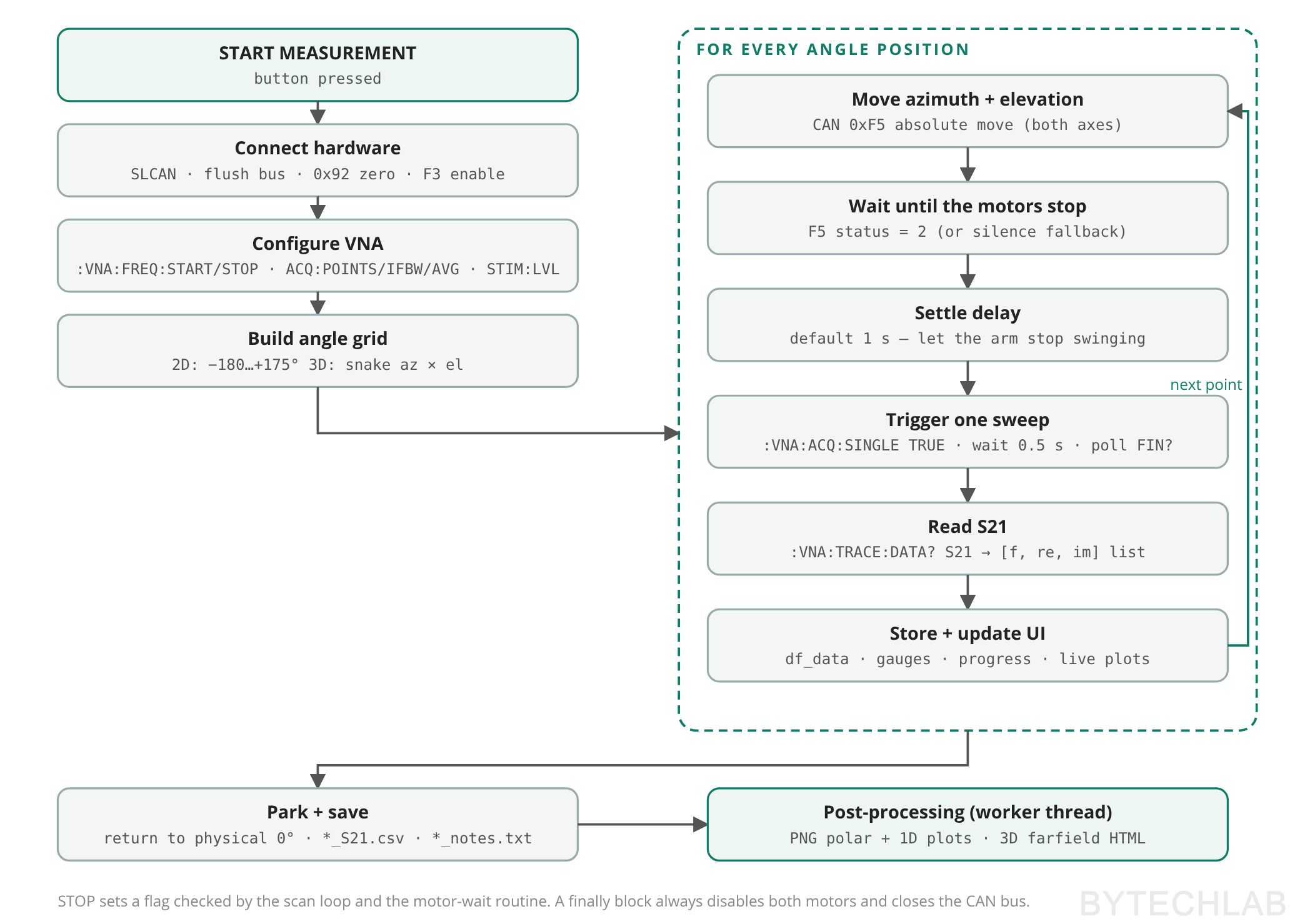
When I press START MEASUREMENT, the script does the following:
- Connect. Opens the CAN bus, flushes old frames, declares the current position of both motors as zero (command 0x92 [4]) and enables them (0xF3).
- Configure the VNA. Sets the mode, the start and stop frequencies, the number of points, averaging, IF bandwidth and output level.
- Build the angle grid. A 2D cut goes from −180° to +175° in the chosen step. A 3D scan does the same in azimuth with elevation from −90° to +90°. On every azimuth column the elevation direction flips (a snake scan), so the motors never have to rewind.
- Measure every point. Sends an absolute move (0xF5) to both motors, waits until they report that they stopped, waits the settle delay, triggers one sweep, polls until it is finished and reads S21. Then it converts S21 to dB, stores it and updates the gauges and plots.
- Finish. Parks the motors at their mechanical zero and saves the CSV and the notes. The polar plots and the 3D HTML are generated in a worker thread, so the GUI stays responsive.
GUI walkthrough
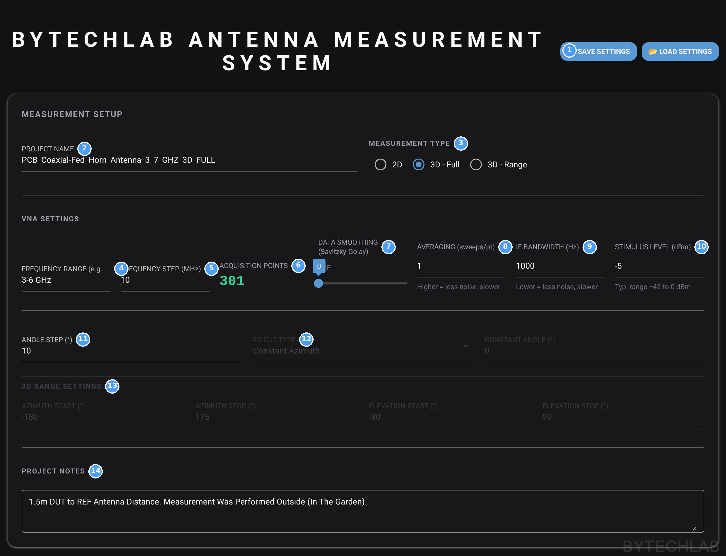
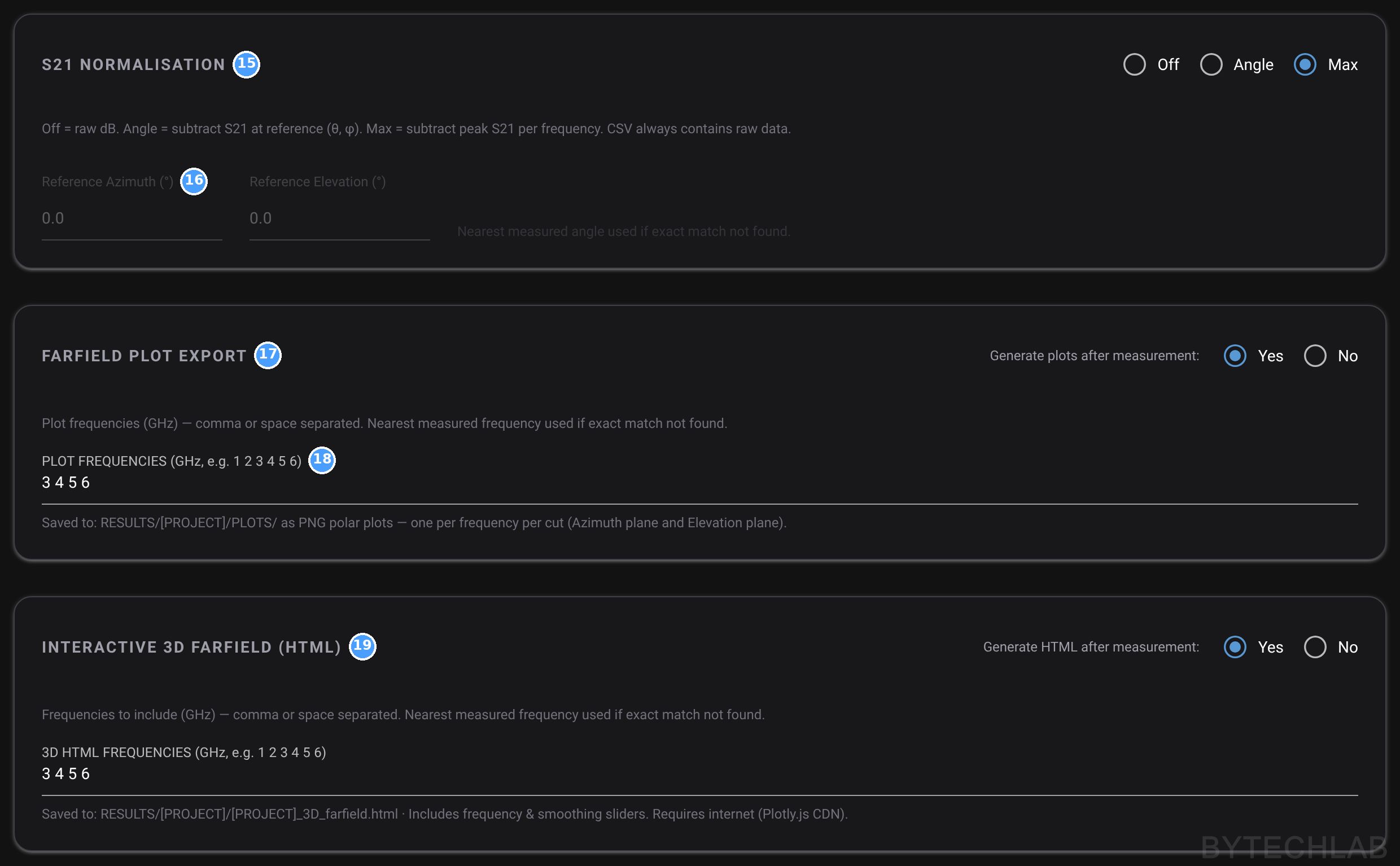
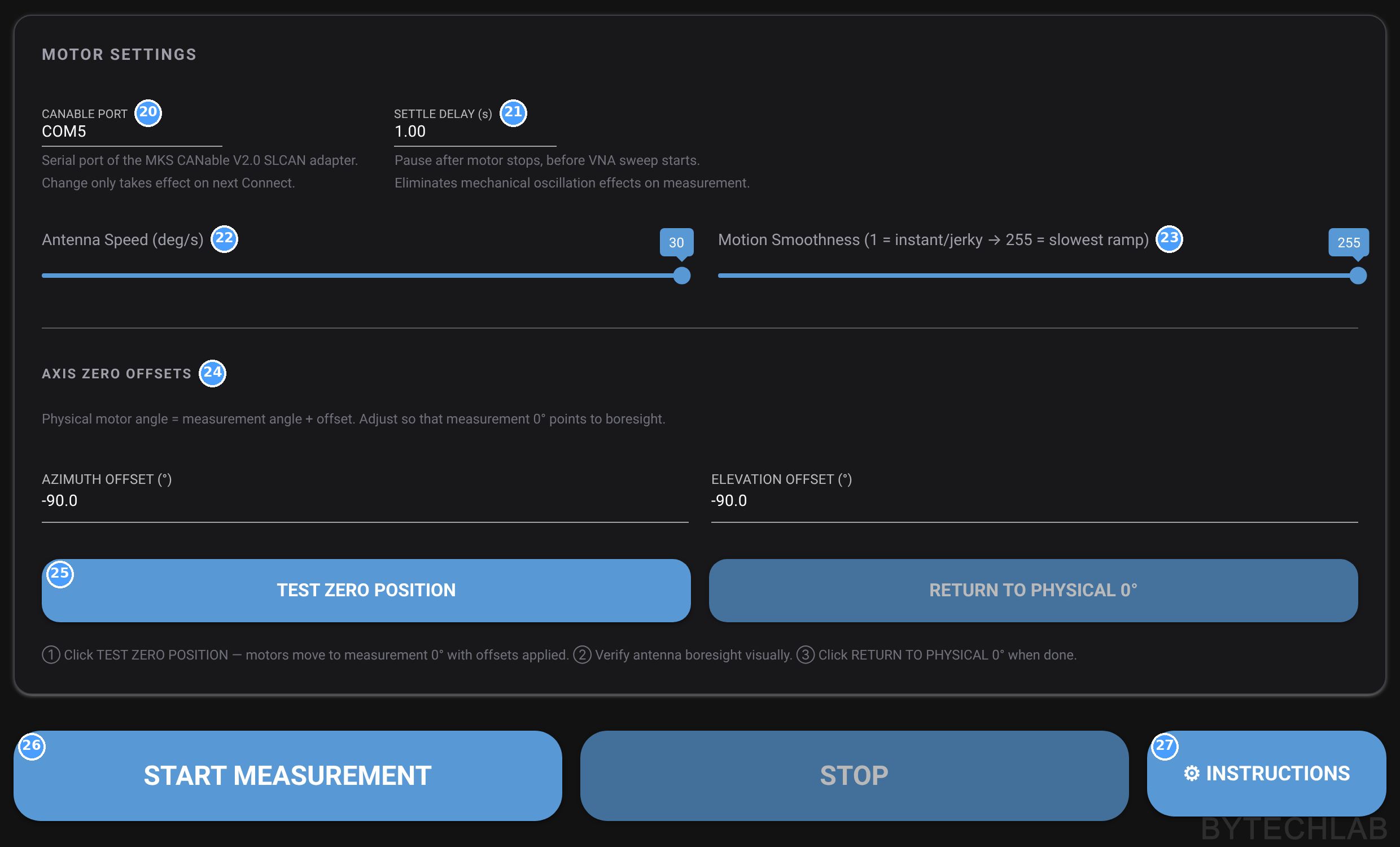
Below are screenshots of the real GUI, taken after measurement of 3D radiation pattern of the PCB horn. The blue numbers match the tables under each picture.
| # | Element | What it does |
|---|---|---|
| 1 | Save / Load settings | Writes every field to antenna_settings.json and reads it back. The file is also loaded automatically when the program starts. |
| 2 | Project name | Name of the results folder RESULTS/<project>/ and prefix of every output file. |
| 3 | Measurement type | 2D (one cut), 3D – Full (whole sphere) or 3D – Range (a limited azimuth/elevation window). |
| 4 | Frequency range | Sweep start–stop in GHz, e.g. “3-6 GHz”. The LibreVNA covers 100 kHz – 6 GHz. |
| 5 | Frequency step | Step in MHz. Together with the range it sets the number of points. |
| 6 | Acquisition points | Computed: (stop − start)/step + 1, limited to 2…10001. 3–6 GHz in 10 MHz steps gives 301. |
| 7 | Data smoothing (Savitzky–Golay) | Optional smoothing of each sweep over frequency, half-window 0–25 points. It is applied before the data is stored, so I keep it at 0. |
| 8 | Averaging | Number of sweeps the VNA averages per point. Less noise, but slower. |
| 9 | IF bandwidth | Narrower = lower noise floor, but a slower sweep. I use 1 kHz. |
| 10 | Stimulus level | Output power of the VNA, typically −42 to 0 dBm. I use −5 dBm. |
| 11 | Angle step | Grid step in degrees, the same for both axes in 3D. |
| 12 | 2D cut type / constant angle | Which axis sweeps in a 2D cut and the fixed angle of the other one. Greyed out in 3D mode. |
| 13 | 3D range settings | Azimuth and elevation start/stop angles for 3D – Range mode. |
| 14 | Project notes | Free text saved to _notes.txt. |
| # | Element | What it does |
|---|---|---|
| 15 | S21 normalisation | Off (raw dB), Angle (S21 at a reference direction is taken as 0 dBi) or Max (the peak (main lobe) is taken as 0 dBi). Only the plots are normalised, the CSV always contains raw data. |
| 16 | Reference azimuth / elevation | Reference direction for Angle mode. The nearest measured point is used. |
| 17 | Farfield plot export | Generate PNG plots automatically after the measurement. |
| 18 | Plot frequencies | List of frequencies in GHz. The nearest measured frequency is used. |
| 19 | Interactive 3D farfield (HTML) | Exports a Plotly 3D HTML file with the radiation pattern for the listed frequencies. |
| # | Element | What it does |
|---|---|---|
| 20 | CANable port | Serial port of the SLCAN adapter (COM5 on my laptop). |
| 21 | Settle delay | Pause after the motors stop and before the sweep, so the boom stops swinging. I use 1 s. |
| 22 | Antenna speed | Axis rotation speed in °/s |
| 23 | Motion smoothness | Acceleration ramp of the MKS motors: acc byte = 256 − value, so 255 is the gentlest ramp. |
| 24 | Axis zero offsets | Physical motor angle = measurement angle + offset. Adjust this so that DUT boresight points to reference antenna. |
| 25 | Test zero / Return to physical 0° | Moves to measurement 0° so I can check that the DUT faces the reference antenna, then back to the mechanical zero. |
| 26 | Start / Stop | Starts or stops the measurement. |
| 27 | Instructions | Motor setup guide, VNA wiring etc.. |
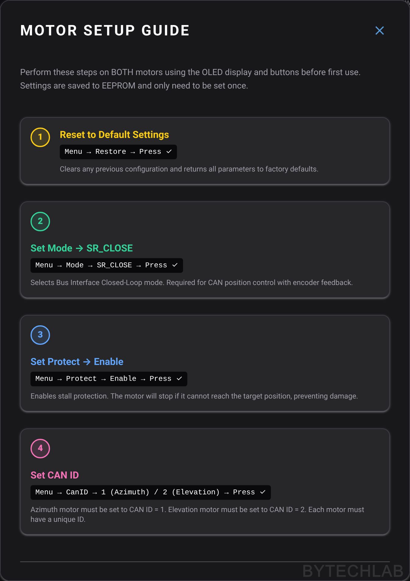
The motors need a one-time setup on their own OLED menu before first use: restore the defaults, select the SR_CLOSE mode (bus control in closed loop with encoder feedback), enable stall protection and set the CAN ID (1 = azimuth, 2 = elevation) [4]. The same dialog shows the VNA wiring (port 1 → reference antenna, port 2 → DUT). It also warns that the two cables together ideally should have less than 10 dB of loss, because the LibreVNA’s dynamic range and port isolation get worse at higher frequencies.
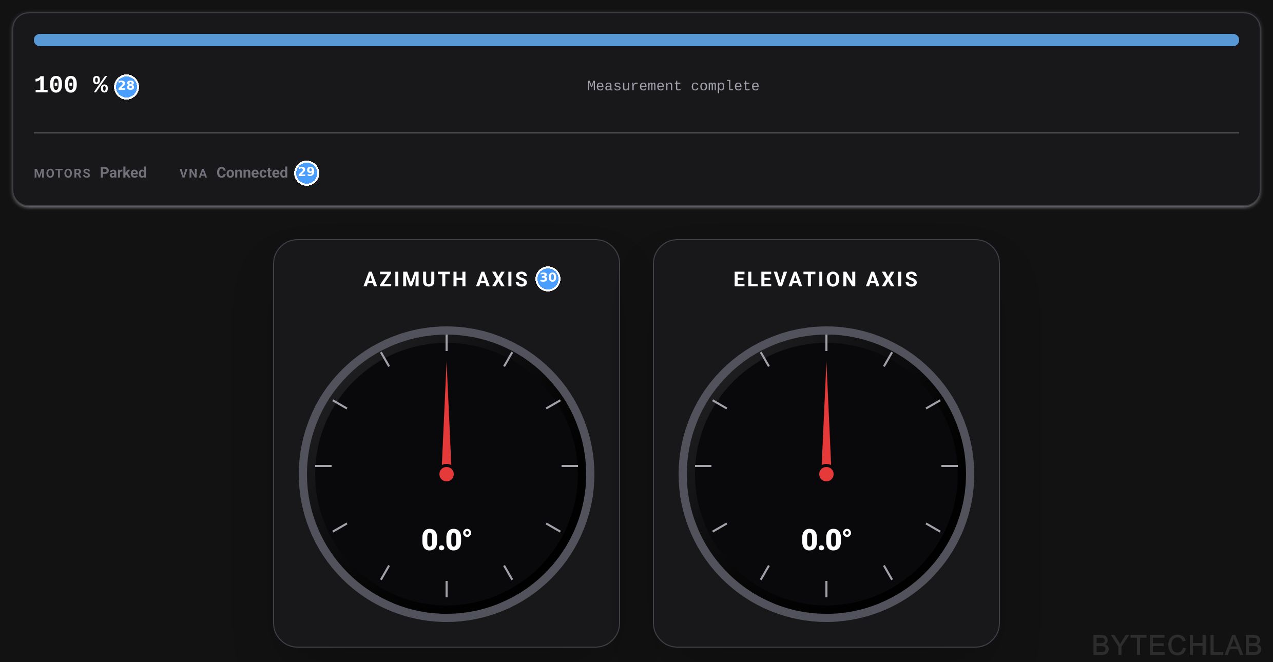
| # | Element | What it does |
|---|---|---|
| 28 | Progress | Percentage, current point and estimated time left. |
| 29 | Motor / VNA status | “Moving…”, “In position”, “Sweeping…”, “Done”, plus VNA error messages if the instrument reports any. |
| 30 | Azimuth / elevation gauges | The current measurement angles of both axes. |
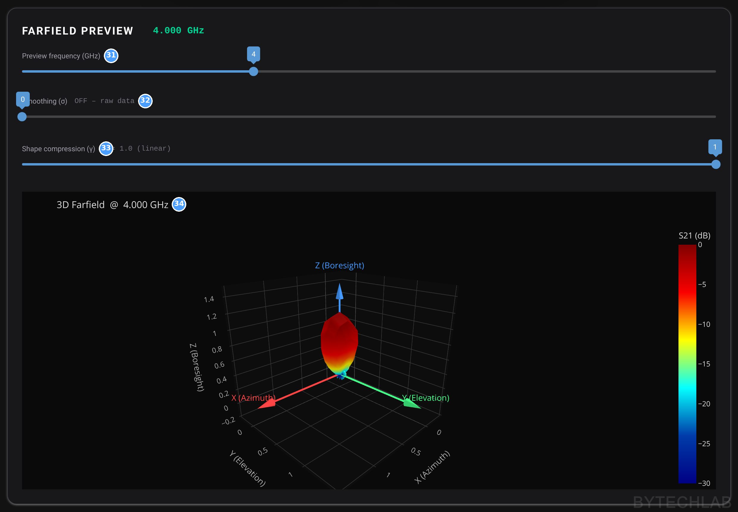
| # | Element | What it does |
|---|---|---|
| 31 | Preview frequency | Which frequency the preview shows. The slider range follows the sweep. |
| 32 | Smoothing σ | Gaussian smoothing of the preview. |
| 33 | Shape compression γ | γ < 1 inflates the weak lobes so the 3D shape is easier to read. Colours stay in dB with a 30 dB window. |
| 34 | 3D farfield preview | Measured pattern as a 3D surface: X lateral, Y up, Z boresight. It updates during the scan. |
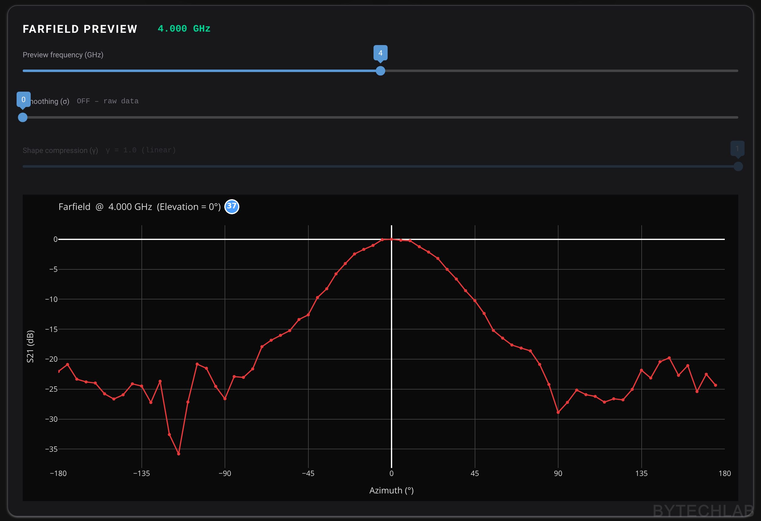
| # | Element | What it does |
|---|---|---|
| 37 | 2D preview | In 2D mode the preview is a cut in dB versus angle, normalised to its peak. |
| # | Element | What it does |
|---|---|---|
| 35 | Live VNA S21 trace | S21 versus frequency at the current point. A quick check that the signal is well above the noise. |
| 36 | Trace plot | Raw dB, before any normalisation. |
Output files
| File | Content |
|---|---|
| RESULTS/<project>/<project>_S21.csv | One row per angle: azim_deg, elev_deg, frequencies, s21_logmag. The last two are space-separated lists (Hz and dB). Always raw, never normalised. |
| <project>_notes.txt | Date and time, all VNA, scan, motor and normalisation settings, and the text notes |
| PLOTS/…_<f>GHz_…_polar.png / _1D.png | For every requested frequency: polar and Cartesian plots of each cut. 3D scans give an azimuth plane and an elevation plane. |
| <project>_3D_farfield.html | Interactive 3D pattern (HTML + Plotly) with frequency, smoothing and shape-compression sliders. 3D modes only, loads Plotly.js from a CDN. |
| antenna_settings.json | All GUI settings (Save / Load buttons) |
Comparison with simulation
A second, smaller script, 10_MEAS_VS_SIM_COMPARISON.py, puts the measured cuts on top of CST far-field exports. It reads the 2D measurement CSVs and the 3D farfield text files exported from the CST. It then builds full ±180° cuts (elevation and azimuth) and shifts every measured cut so that the main lobes from the simulation and measurement point to the same direction. After 5-point Savitzky–Golay smoothing over angle, it computes the RMS difference in dB. It saves one polar plot per frequency and cut, with a coloured RMS badge.
Video
On the video above you can see the measurement process (for 2D and 3D radiation patterns).
5) Photos
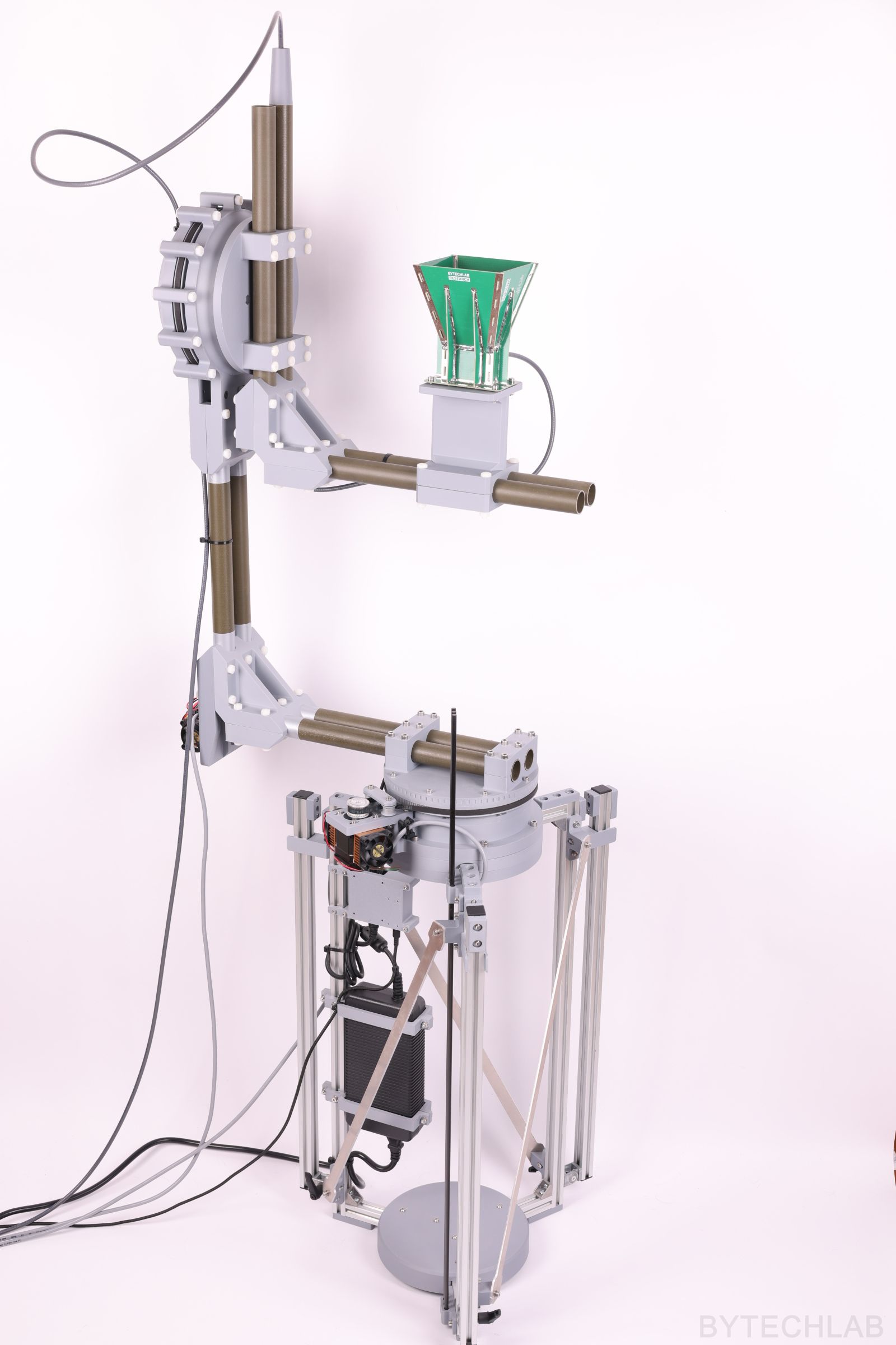
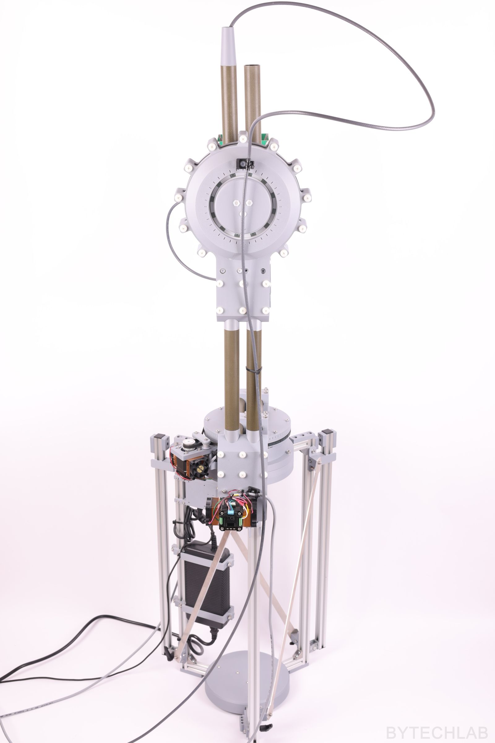
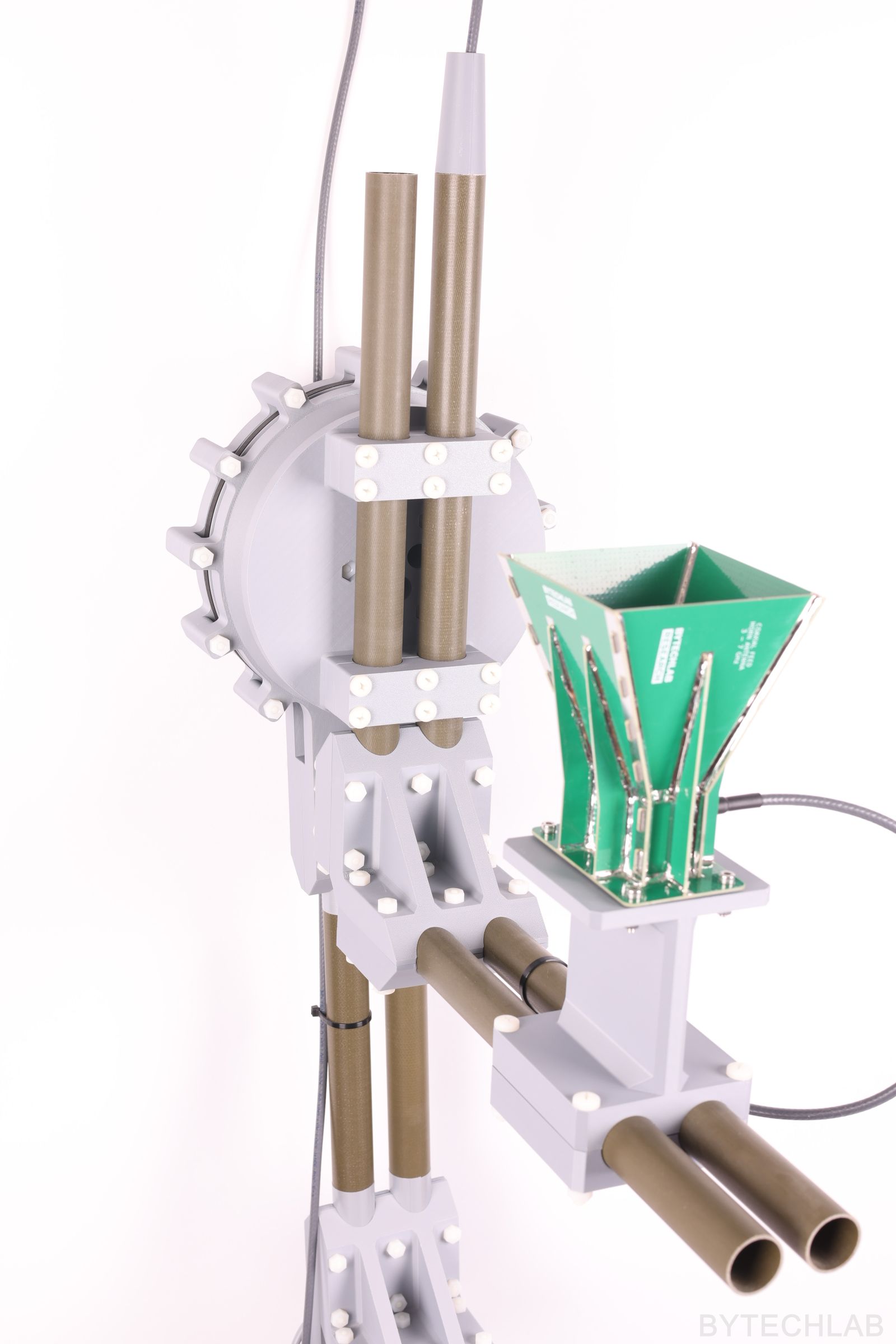
On the photos above and below you can see the finished antenna positioner.
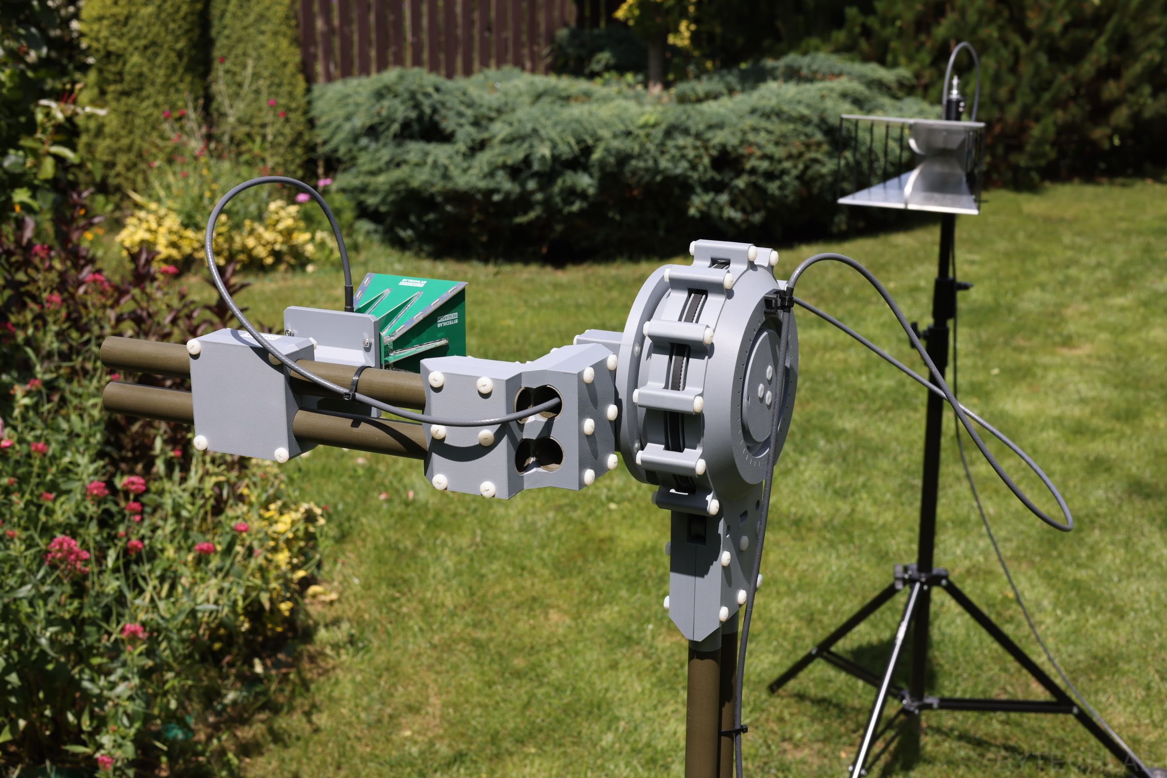
The grey parts are printed in PLA, the olive tubes are fiberglass and the white heads all around the joints are nylon screws. The electronics box with the CANable sits on the frame below the azimuth joint, next to the power brick.
6) Measurements
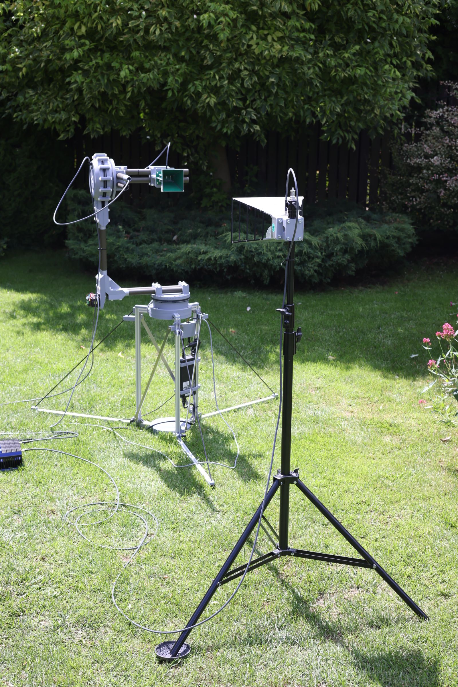
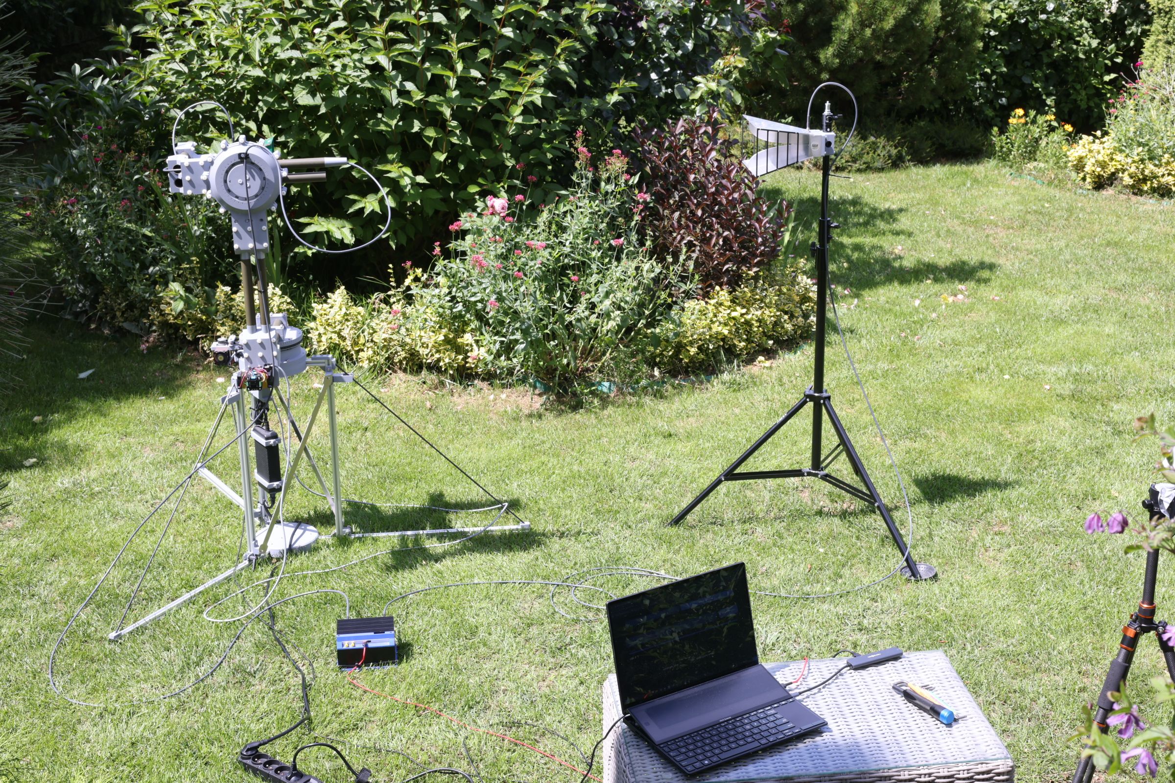
All measurements were done in my garden. The reference DRH stands on a photo tripod. The positioner stands about 1.5 m away, and both antennas are about 1.25 m above the grass. The laptop that controls everything sits on a small table behind the positioner.
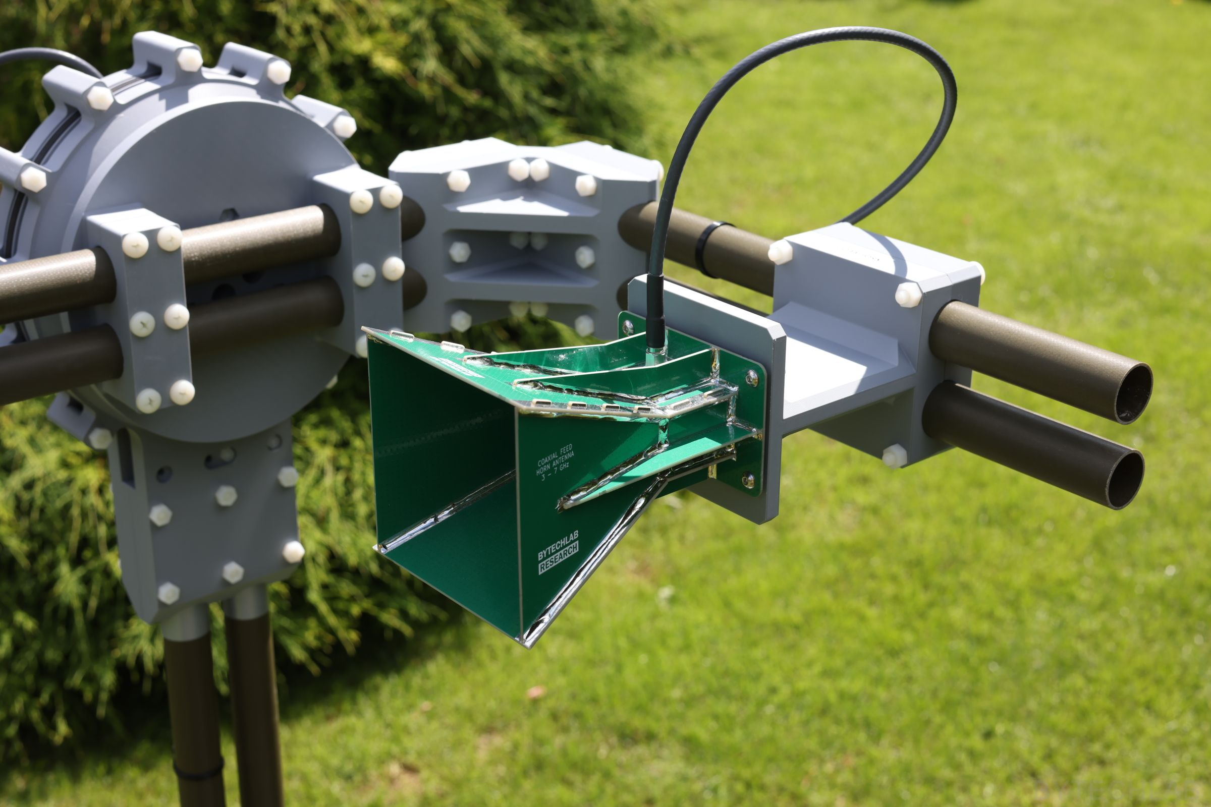
I measured two of my antennas: the PCB coaxial-fed horn (3–7 GHz) and the 3D-printed double-ridged horn (2–6 GHz). Both have CST models, so I can compare the measured cuts with simulated far-field cuts. Settings:
- 3–6 GHz in 10 MHz steps (301 points) for the PCB horn, 2–6 GHz for the DRH
- IF bandwidth 1 kHz, −5 dBm, no averaging, settle delay 1 s
- 5° steps for the 2D cuts, 10° for the 3D scans
The plots below compare the two 2D cuts of the PCB horn with the CST cuts (elevation and azimuth). The RMS difference is computed in dB on a 1° grid, with both curves clipped at −30 dBi so the noise floor doesn’t dominate. The badge is green up to 3 dB, amber up to 6 dB and red above.
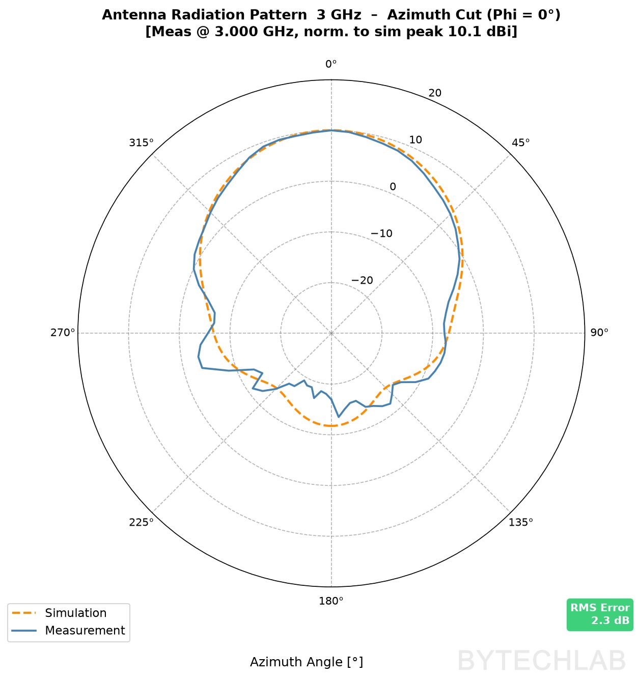
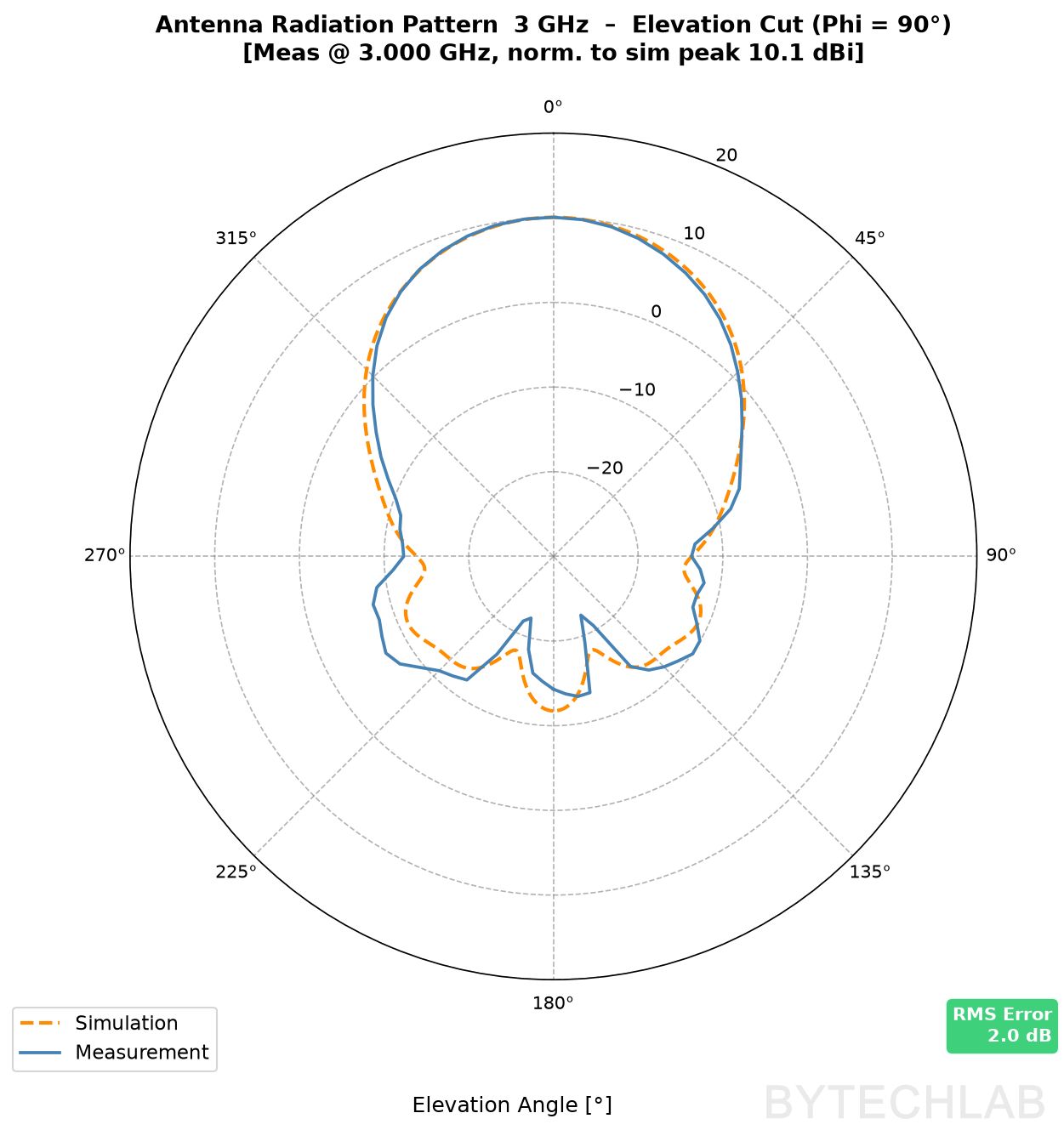
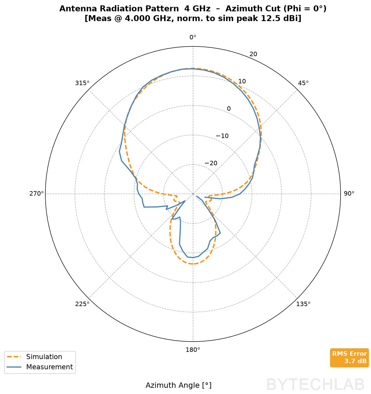
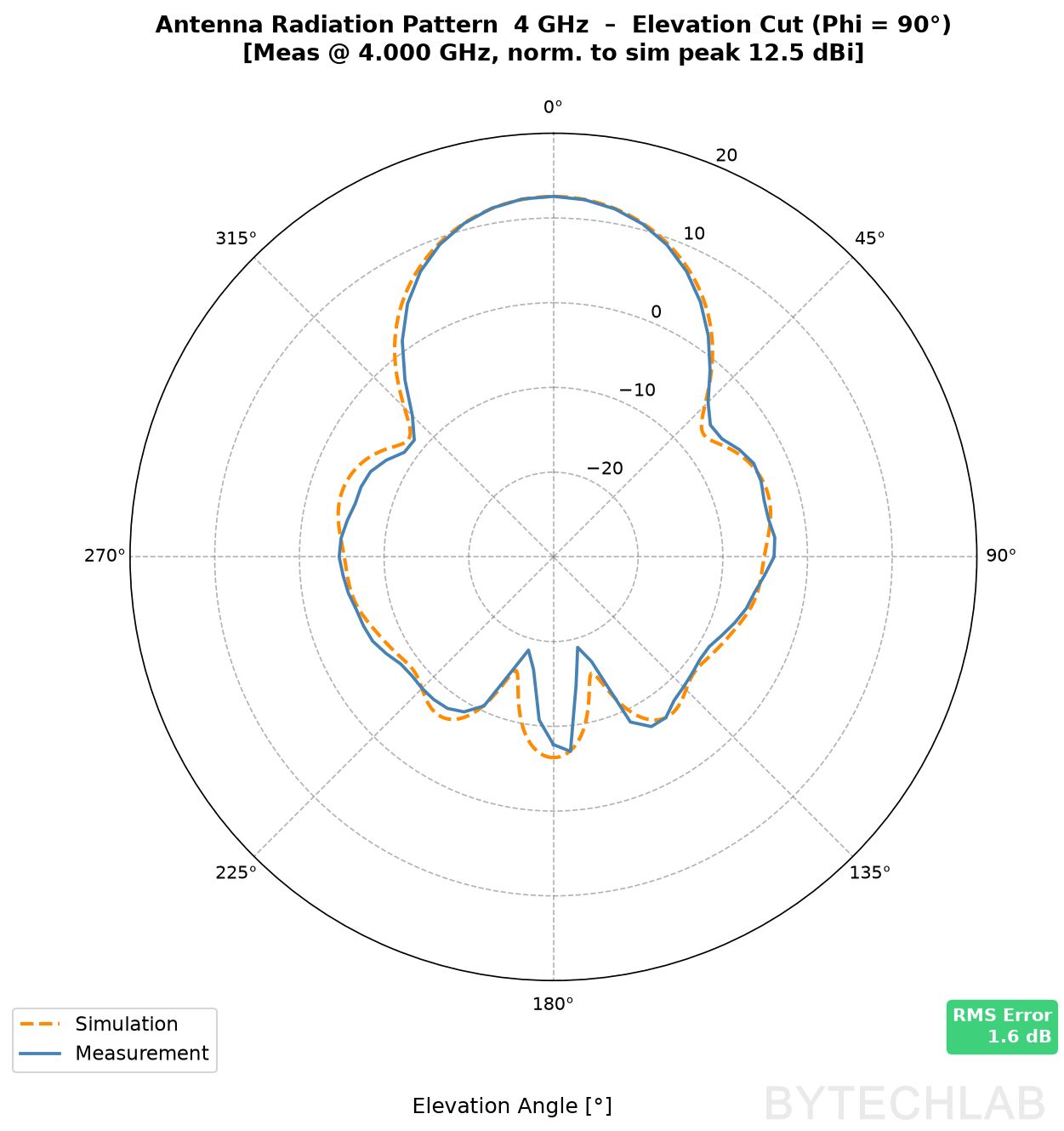
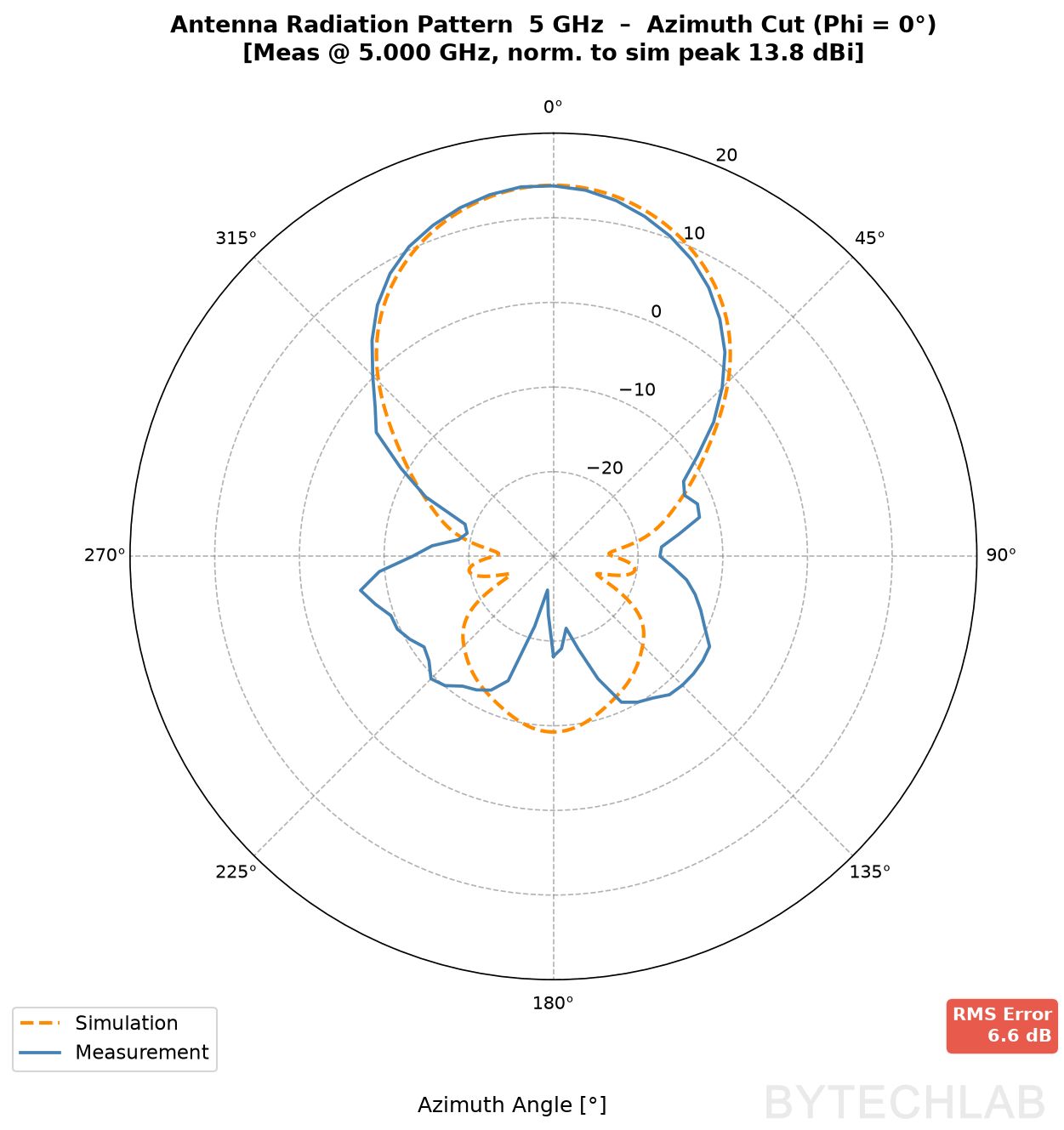
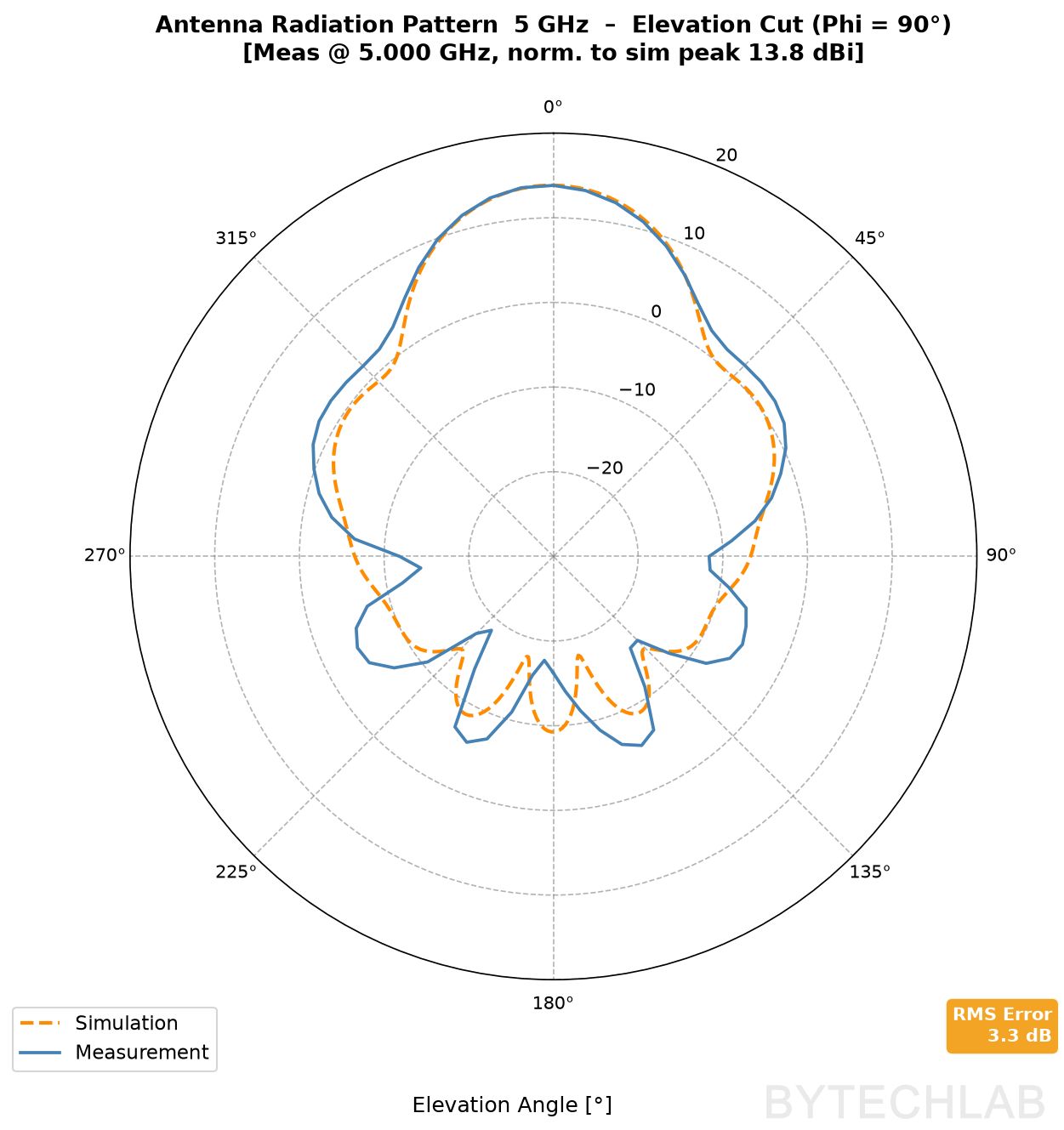
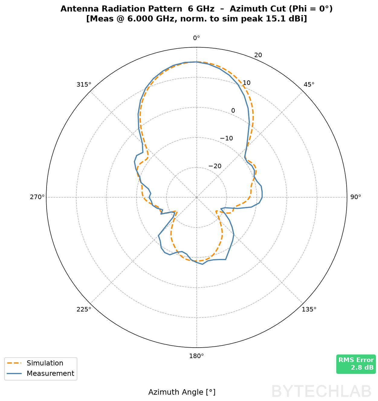
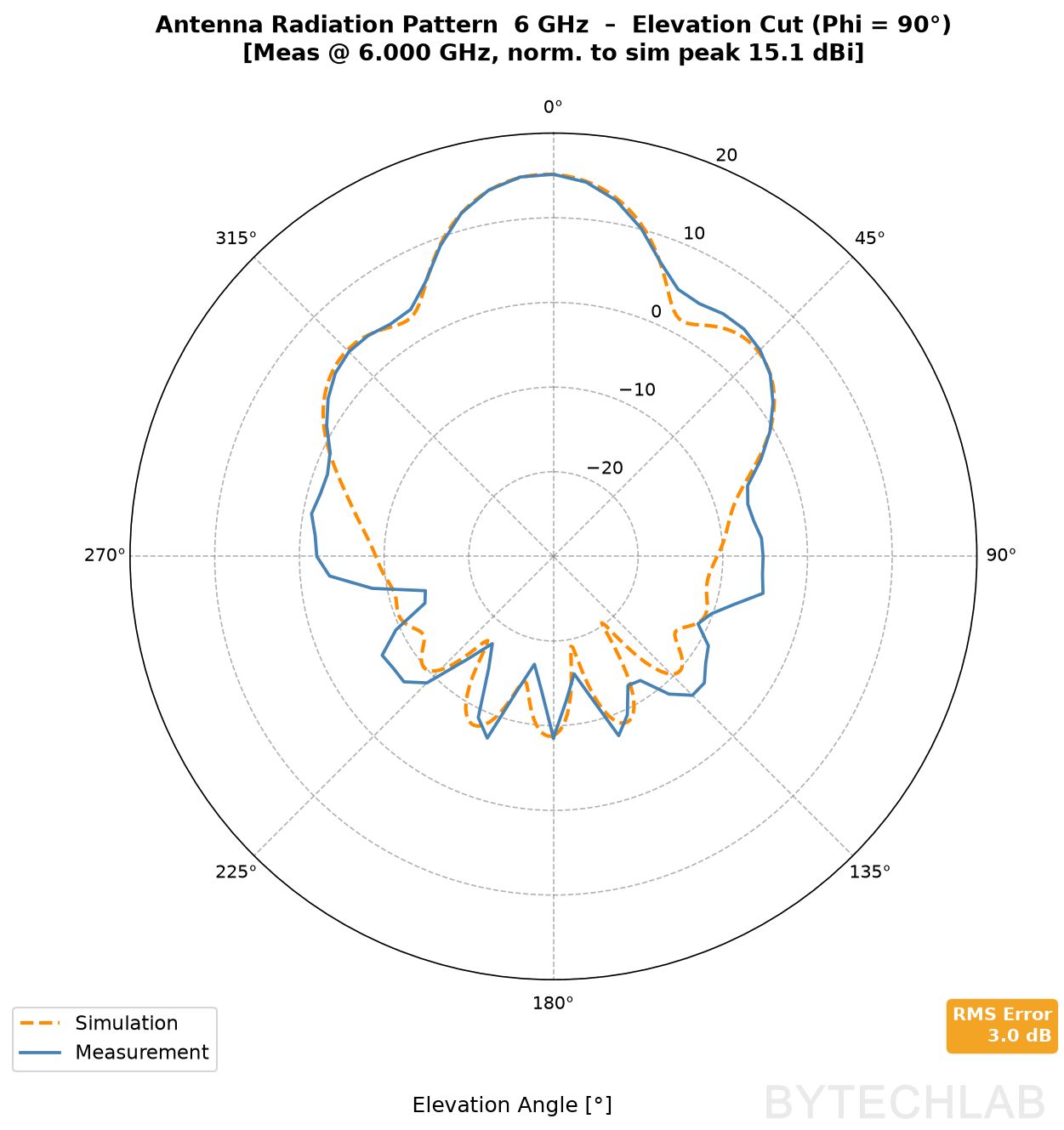
The main lobes match well at all frequencies. The differences are in the side and back lobes, 20–30 dB down, where every echo from the ground, the tripods or the garden matters (see equation (5)). The elevation cuts of the PCB horn are within 1.6–3.3 dB RMS. The worst case is the azimuth cut at 5 GHz with 6.6 dB.
Interestingly, the 3D-printed DRH is also worst in the azimuth cut at 5 GHz (5.4 dB). When two different antennas fail at the same frequency and in the same cut, that points to the measurement setup rather than to the antennas.
| Antenna | Cut | 2 GHz | 3 GHz | 4 GHz | 5 GHz | 6 GHz |
|---|---|---|---|---|---|---|
| PCB coax-fed horn | azimuth (φ = 0°) | – | 2.3 | 3.7 | 6.6 | 2.8 |
| elevation (φ = 90°) | – | 2.0 | 1.6 | 3.3 | 3.0 | |
| 3D-printed DRH | azimuth (φ = 0°) | 2.7 | 1.9 | 1.8 | 5.4 | 3.8 |
| elevation (φ = 90°) | 1.9 | 2.3 | 1.7 | 3.0 | 2.8 |
On the video below you can see how the antenna positioner rotates the antenna:
Below you can find the real measured interactive 3D radiation pattern that you can rotate with your mouse!
What limits the accuracy
- Echoes from the ground, the tripods, the table and the garden. They mostly affect sidelobes and back lobes (eq. (5)). Time gating would remove most of them, but needs complex S21.
- Distance. 1.5 m is enough for the DUT, but short for the large reference horn at 5–6 GHz , I will increase this distance in the future,
- Alignment. Zero offsets are set by eye with TEST ZERO POSITION. A few degrees of error shift the whole cut.
- The positioner itself. The dielectric upper part still scatters a little, and the metal lower also interacts with the DUT for some of the angles (EM absorbers would help here)
7) Specifications
| Configuration | Elevation-over-azimuth, 2 axes |
| Angular range | Azimuth −180…+175°, elevation −90…+90° (full sphere) |
| Drive | 2× MKS SERVO42D CAN, HTD3M belts 8:1 (azimuth), 10:1 (elevation) |
| VNA | LibreVNA, 100 kHz – 6 GHz, S21 |
| Typical scan duration | 2D cut: 72 stops (5°), a few minutes · 3D: 684 stops (10°), under 1 hour |
| Test range | Outdoor, open field |
| Software | Python: NiceGUI, python-can, NumPy, pandas, SciPy, Matplotlib, Plotly |
| Outputs | CSV, notes TXT, PNG polar/1D plots, interactive 3D HTML |
8) Conclusions
The positioner does what I wanted. I can take an antenna into the garden, press start, and come back to a full set of 2D cuts and a 3D pattern that I can compare with the simulation. For the main lobe and the first sidelobes, the agreement with CST is 2–4 dB RMS at most frequencies. That is good enough to tell whether a design behaves like its model. Below about −20 dB, the garden takes over.
This setup will be ideal for phased array prototyping / debugging ( I will change phases and amplitudes at each element to fine tune the array ). Instead of going into a professional lab with anechoic chamber every time I can simply do most of the preliminary measurements on-site which is huge time saver.
What I want to improve next:
- store complex S21, so I can time-gate the ground echo [2], [3]
- measure absolute gain with a gain-transfer or three-antenna measurement [1], [2]
- put some absorbers in the appropriate places
9) References
- [1] C. A. Balanis, Antenna Theory: Analysis and Design, 4th ed., Wiley, 2016.
- [2] IEEE Recommended Practice for Antenna Measurements, IEEE Std 149-2021, 2022.
- [3] J. Olencki, V. Waladi, A. Bekasiewicz and L. Leifsson, “A low-cost system for far-field non-anechoic measurements of antenna performance figures,” IEEE Access, vol. 11, pp. 39165–39175, 2023, doi: 10.1109/ACCESS.2023.3268116.
- [4] Makerbase, MKS SERVO42D/57D_CAN User Manual, V1.0.3.
- [5] LibreVNA SCPI Programming Guide, LibreVNA project, https://github.com/jankae/LibreVNA.